
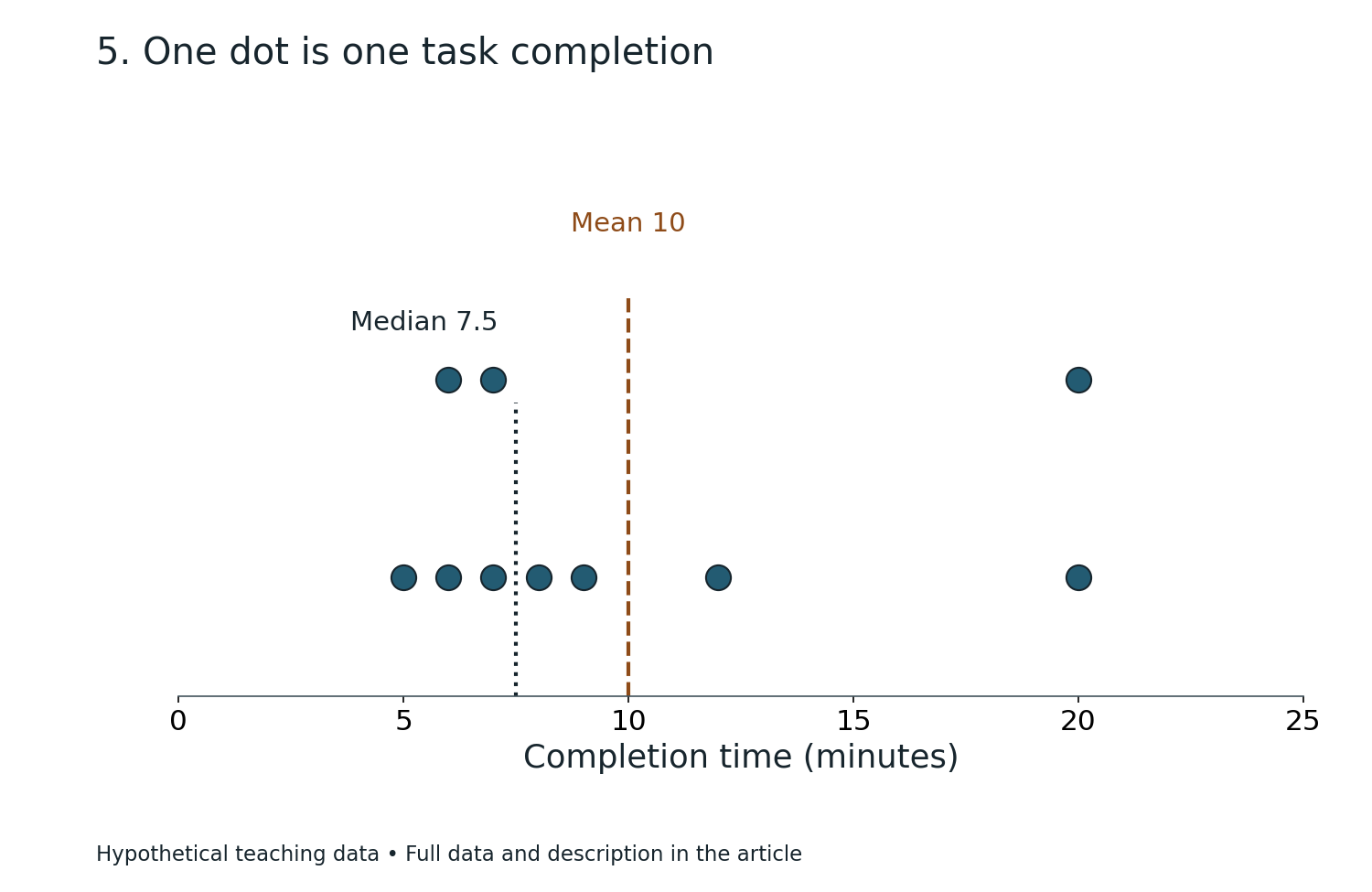
Two fictional students each record eight reading-session durations. One student’s schedule includes a very long session, while the other’s stays fairly consistent. Their averages alone do not tell the full story. Quartiles and box plots can show where the middle half of the observations lies, how widely the values are spread and whether any recorded day is unusually far from the rest.
This Mathematics in Bukit Timah guide uses completely invented reading-session data, not measurements from local children, families, schools or tuition centres. The neighbourhood provides a familiar educational setting; the statistics follow from the defined datasets. The lesson develops ordering, median, lower and upper quartiles, interquartile range (IQR), box-and-whisker diagrams, outlier conventions and responsible interpretation.
The quick example is a sorted eight-session dataset: 10, 12, 14, 15, 18, 20, 22, 40 minutes. Under the median-of-halves convention used throughout this article, the median is 16.5, lower quartile Q1 is 13, upper quartile Q3 is 21, and IQR = 21−13 = 8 minutes. The minimum is 10 and maximum 40. The unusually large value 40 deserves examination, not automatic removal.
Article contents
- Quick answer: the median of halves creates the quartiles
- Why Bukit Timah is a setting and not a survey
- Begin with the order of observations
- Worked example 1: calculate the complete five-number summary
- The word quartile depends on a calculation convention
- Why eight records make a clean teaching example
- Worked example 2: confirm the median and quartiles with positions
- The IQR measures the middle half’s spread
- Worked example 3: alter only the last duration
- Range and IQR should not be confused
- A box plot uses the quartile positions as geometry
- Two common whisker conventions must be distinguished
- Worked example 4: draw the simple five-number box plot
- An outlier rule must be stated before it is used
- Worked example 5: modified box plot with a separate outlier
- Why a flagged outlier must be investigated rather than erased
- Worked example 6: calculate the mean before and after alteration
- A second fictional group makes comparison meaningful
- Worked example 7: compare the two medians
- Worked example 8: compare outlier fences for B
- Comparing box plots requires a common axis
- What does a longer box mean?
- Worked example 9: same median, different spread
- The median line need not divide the box visually in half
- Worked example 10: an off-centre median
- Five-number summaries do not recover every observation
- Worked example 11: why the maximum may dominate one whisker
- Quartiles and percentiles are related concepts
- Why software can display different quartiles
- Quartile methods and odd-sized datasets
- Worked example 12: use a clearly defined nine-value convention
- IQR has the same unit as the recorded variable
- A box plot does not show sample size unless labelled
- Worked example 13: equal box lengths, different numbers of observations
- Outliers and skew are different concepts
- The box plot and histogram provide different perspectives
- Worked example 14: when unequal histogram bins complicate comparison
- Weighted averages and quartiles answer different questions
- Worked example 15: recover dataset B’s mean
- Do not label the longest session a failure
- A real study log must define the recorded unit
- Missing data are not zeros
- Quartiles from percentages do not imply causal improvement
- A tutor should diagnose the earliest invalid step
- Worked example 16: correct a mistaken Q3
- Primary preparation: order and middle values first
- Upper Primary: connect range with variability
- G3 Secondary Mathematics: box-and-whisker interpretation
- Upper Secondary extension: infer cautiously from samples
- A twenty-minute home diagnostic
- A seven-day practice plan with retrieval
- Five challenge questions and model answers
- Frequently asked questions
- Official curriculum context and connected learning

Quick answer: the median of halves creates the quartiles
Quartiles divide ordered data into lower and upper portions. Under a common school method, find the overall median, then find the median of the lower half for Q1 and the median of the upper half for Q3.
For eight values, the first four form the lower half and the last four form the upper half. From 10,12,14,15,18,20,22,40, the lower-half median is (12+14)/2=13.
The upper-half median is (20+22)/2=21. The interquartile range is 21−13=8. This summary focuses on the middle half of the dataset rather than the extreme endpoints.
Why Bukit Timah is a setting and not a survey
A family around Beauty World, Sixth Avenue or King Albert Park can understand a personal study log, revision record or series of fictional reading sessions. No neighbourhood statistic needs to be invented for the Mathematics to be meaningful.
A descriptive chart is only as factual as the observations that created it. In this lesson, every observation is fabricated for clear working, so no result should be generalised to real Bukit Timah students.
The goal is to make children ask which quantity a summary describes, how it was calculated and whether the evidence supports a broader conclusion.
Begin with the order of observations
Imagine eight durations written in the order 22,10,40,15,18,12,20,14. This order may reflect when a fictional student entered them, but it is not suitable for finding positional quartiles directly.
Sort them into 10,12,14,15,18,20,22,40. Now the fourth and fifth observations are 15 and 18.
Their average gives overall median 16.5. A student who takes the central numbers of the original unsorted list has not followed the mathematical median definition.
Worked example 1: calculate the complete five-number summary
For the sorted dataset A, minimum is 10, Q1 is 13, median is 16.5, Q3 is 21 and maximum is 40, all measured in minutes.
These five statistics are called the five-number summary. They are intended to convey position and spread without showing all eight original records individually.
The full range is 40−10=30 minutes. The interquartile range is 21−13=8 minutes. Range and IQR differ because they describe different parts of the distribution.
The word quartile depends on a calculation convention
Several quartile definitions exist. Software and school materials sometimes use interpolation or different rules for handling a median when the number of observations is odd.
This article consistently uses the median-of-halves method, with the full dataset split into equal lower and upper halves when the count is even. Other conventions can produce slightly different Q1 and Q3 for the same data.
When solving an examination question, follow the definition or method specified in the relevant syllabus, question or class. Do not silently combine outputs from different quartile methods.
Why eight records make a clean teaching example
An even dataset of eight observations splits into four lower values and four upper values without debating how to handle a central observation inside either half.
Each quartile is the mean of the two central values in its half. That is why Q1=13 arises from 12 and 14 rather than being selected automatically from a single recorded duration.
The quartile values do not have to appear in the raw dataset. Like the mean or overall median, they can lie between observed values.
Worked example 2: confirm the median and quartiles with positions
Sorted positions one through eight contain 10,12,14,15,18,20,22,40. The overall median is the average of positions four and five: 16.5.
Lower half positions one through four have central values 12 and 14, producing Q1=13. Upper half positions five through eight have central values 20 and 22, producing Q3=21.
The positional reasoning is more reliable than memorising “divide by four” without stating the quartile convention.
The IQR measures the middle half’s spread
The interquartile range is Q3−Q1. It measures the width of the interval between the lower and upper quartiles.
In dataset A, that middle interval runs from 13 to 21 minutes, with width eight minutes. It does not claim that every observation lies inside that interval.
Compared with the full range, IQR is often less affected by a single extreme value. It uses quartile positions rather than only the smallest and largest records.
Worked example 3: alter only the last duration
Replace the invented 40-minute session with 24 minutes, producing 10,12,14,15,18,20,22,24.
The overall median remains 16.5, Q1 remains 13 and Q3 remains 21, so IQR is still eight minutes. But the maximum changes from 40 to 24 and the range falls from thirty to fourteen minutes.
This is a concrete example of how an extreme value can change the range while leaving the quartiles unchanged under the stated dataset and convention.
Range and IQR should not be confused
Range is maximum minus minimum. IQR is upper quartile minus lower quartile. Both have the original variable’s units.
For dataset A, the results are range 30 minutes and IQR 8 minutes. Reporting IQR as 30 would substitute extreme spread for middle spread.
A pupil should be able to state which two values are subtracted in each calculation and show them on a number line.
A box plot uses the quartile positions as geometry
A conventional box-and-whisker plot displays a box from Q1 to Q3, a line marking the median inside the box and whiskers showing the appropriate endpoints under the chosen plot convention.
The box width along a horizontal numerical axis therefore represents IQR. In dataset A, the box begins at 13 and ends at 21, with the median marked at 16.5.
Every plotted position is based on the variable’s numeric scale. The heights or decorative thickness of boxes are not the values being compared.
Two common whisker conventions must be distinguished
A simple five-number-summary box plot extends whiskers to the actual minimum and maximum. Under that style, dataset A’s whiskers reach 10 and 40.
A modified box plot may instead use a specified outlier rule, drawing whiskers to the most extreme observations not classified as outliers and plotting outliers separately.
The two plots can represent the same observations while drawing different whiskers. A reader should check which convention is being used before interpreting the diagram.
Worked example 4: draw the simple five-number box plot
Under a simple min–max whisker convention, draw a box from 13 to 21 and a median mark at 16.5.
Extend the left whisker to the minimum 10 and the right whisker to maximum 40. Label the axis as reading-session duration in minutes.
The right whisker is much longer than the left, suggesting that the upper side extends farther. The graph reports the eight invented records, not a typical profile of real children.
An outlier rule must be stated before it is used
A common exploratory convention marks observations lying below Q1−1.5×IQR or above Q3+1.5×IQR as potential outliers.
For dataset A, IQR is eight, so 1.5×IQR=12. The lower fence is 13−12=1, and the upper fence is 21+12=33.
The invented value 40 lies above 33. Under this stated convention, 40 is flagged as a potential outlier. Being flagged does not automatically mean it is wrong.
Worked example 5: modified box plot with a separate outlier
The sorted durations are 10,12,14,15,18,20,22,40. Under the 1.5×IQR rule, all values except 40 lie between fences 1 and 33.
The modified whiskers reach the smallest and largest non-outlier observations, 10 and 22. The value 40 appears as a separate point beyond the right whisker.
If a pupil draws the modified right whisker to the fence 33 instead of observed value 22, they have used the fence as though it were an actual record. In this convention the whisker ends at the extreme non-outlier observation.
Why a flagged outlier must be investigated rather than erased
Forty minutes might represent a genuine longer session. It could also reflect an entry error, an interruption rule or a different definition of “reading”.
The statistical fence identifies a value worth examining. It does not demonstrate that the record is false or unsuitable for the analysis.
A responsible explanation may show the summary with and without the value, while retaining and documenting the underlying observation unless there is a defensible reason to change it.
Worked example 6: calculate the mean before and after alteration
For dataset A, total minutes are 10+12+14+15+18+20+22+40=151. Mean is 151/8=18.875 minutes.
After replacing 40 with 24 in a different hypothetical dataset, total becomes 135 and mean 135/8=16.875 minutes.
The mean changes by two minutes while the quartiles and IQR remain fixed in this example. This shows why a descriptive report may include measures of both centre and spread.
A second fictional group makes comparison meaningful
Consider dataset B: 13,14,14,15,17,18,19,20 minutes. It also contains eight invented observations.
Its median is (15+17)/2=16. Its lower quartile is (14+14)/2=14. Its upper quartile is (18+19)/2=18.5.
Therefore B’s IQR is 18.5−14=4.5 minutes and its range is 20−13=7 minutes. The values are more tightly grouped than A’s under these measures.
Worked example 7: compare the two medians
Dataset A has median 16.5 minutes. Dataset B has median 16 minutes. The difference is only half a minute.
This small median difference does not mean the distributions are almost identical. Their IQRs are eight and 4.5, and their ranges are thirty and seven.
A good comparison states both a measure of centre and a measure of spread instead of treating one central number as a full description.
Worked example 8: compare outlier fences for B
For dataset B, Q1=14, Q3=18.5 and IQR=4.5. The multiplier 1.5×IQR is 6.75.
The lower fence is 14−6.75=7.25; the upper is 18.5+6.75=25.25. All observed values from 13 to 20 lie inside, so none is flagged by this rule.
That conclusion belongs to dataset B and the selected convention. It does not prove there could never be an outlier in a larger sample from the same imaginary process.
Comparing box plots requires a common axis
Place the two box plots on the same numerical horizontal scale. Otherwise, a box occupying ten centimetres on one drawing may be numerically narrower than a small-looking box on another chart with a different scale.
Label the units and tick marks. Readers should compare coordinates, not pixel widths.
This is especially important in educational reports where cropped axes or mismatched scales can make one learner’s variation appear more extreme or less extreme than it really is.
What does a longer box mean?
A longer box represents a larger IQR on the displayed numerical scale. It indicates the middle half spans a wider range of values.
It does not necessarily mean a higher mean, more total observations or lower quality of performance. The meaning depends on the quantity being studied and the context.
Two groups can have identical IQRs with different medians. They can also have identical medians with different IQRs.
Worked example 9: same median, different spread
Imagine X: 8,9,10,10,10,10,11,12 and Y: 0,2,8,10,10,12,18,20.
Both have median ten. For X, Q1=(9+10)/2=9.5 and Q3=(10+11)/2=10.5, giving IQR one. For Y, Q1=(2+8)/2=5 and Q3=(12+18)/2=15, giving IQR ten.
The same median conceals a tenfold difference in IQR. It is an illustration of why central tendency alone is insufficient.
The median line need not divide the box visually in half
In a box plot, Q1 and Q3 mark quartiles but the median may lie nearer one end of the box when the observations are asymmetrically distributed.
That position can suggest uneven distribution within the middle half. It does not directly prove a specific causal mechanism or a unique distribution shape.
The box plot compresses data, so many different raw datasets can share the same five-number summary. A cautious interpretation acknowledges information lost in the summary.
Worked example 10: an off-centre median
Take fictional sorted data 2,3,4,4,5,6,12,20. Under median-of-halves, Q1=(3+4)/2=3.5, median=(4+5)/2=4.5 and Q3=(6+12)/2=9.
The median lies only one unit above Q1 but 4.5 units below Q3. The right half of the box is much longer.
The skewed box segment suggests uneven spread among the observations, but the exact raw values still matter for a complete description.
Five-number summaries do not recover every observation
Suppose two datasets have the same minimum, Q1, median, Q3 and maximum. Their middle values can still differ.
A box plot does not reveal exactly how many repeated values occur within a quartile interval, where every non-quartile point lies, or the precise mean.
This is a limitation of statistical compression rather than a defect. A good chart makes its strengths and omissions understood.
Worked example 11: why the maximum may dominate one whisker
Dataset A’s maximum is 40 and the next-highest value is 22. Under min–max whiskers the right whisker extends from Q3=21 to 40, a length of nineteen minutes.
Under the modified box plot, the right whisker extends only to 22 because 40 is plotted separately. The box, quartiles and median are unchanged.
The visualization differs because the whisker convention differs. Always state which convention a comparison uses.
Quartiles and percentiles are related concepts
Under commonly used definitions, Q1 corresponds approximately to the twenty-fifth percentile, the median to the fiftieth and Q3 to the seventy-fifth.
The word “approximately” matters because different finite-sample quantile conventions may interpolate differently. A percentile is a position-based summary of ordered values.
When a school question specifies a quartile convention, use that rule rather than mixing it with the default quantile function from an unrelated spreadsheet package.
Why software can display different quartiles
Some programs use percentile interpolation rules based on fractional ranks, whereas a school solution may split the observations into lower and upper halves.
For small datasets, those methods can yield different numerical quartiles without either implementation containing an arithmetic mistake.
To compare results fairly, record the method, sample count, and any interpolation convention. Reproducibility begins with identifying the calculation definition.
Quartile methods and odd-sized datasets
Suppose an imaginary dataset has nine ordered values. Some median-of-halves teaching approaches exclude the overall median from the lower and upper halves, while other conventions include it or interpolate.
That distinction can change Q1 or Q3. It is better to show an explicit school rule than to assert one universal formula for all odd dataset sizes.
The eight-value examples in this article avoid that particular ambiguity while illustrating the key box-plot structure and IQR reasoning.
Worked example 12: use a clearly defined nine-value convention
Take sorted values 2,4,6,8,10,12,14,16,18. Suppose the instruction says to exclude the overall median when finding quartiles.
Median is 10. The lower half 2,4,6,8 has Q1=(4+6)/2=5. The upper half 12,14,16,18 has Q3=(14+16)/2=15.
IQR is ten. The answer is correct under the named convention. If a different convention is mandated, recompute accordingly.
IQR has the same unit as the recorded variable
If a dataset consists of minutes, Q1, Q3 and IQR are in minutes. If it consists of test scores, they are in score points.
The IQR is a difference of two observations on the same numerical scale. It is not automatically a percentage or a count of students.
To report IQR as a percentage, a separate and justified denominator would need to be specified. Adding a percent sign because the word “quartile” suggests four parts is incorrect.
A box plot does not show sample size unless labelled
Two groups may each have a box drawn with the same visual thickness, even if one contains eight observations and the other eighty.
The standard box plot’s width usually does not encode sample size unless a specialised convention explicitly does so. A responsible comparison labels n separately.
This is important for parents reading dashboards: a tight box based on only a few records should not be mistaken for evidence about an entire school population.
Worked example 13: equal box lengths, different numbers of observations
Imagine group C with eight observations and group D with eighty observations. Both are constructed so their Q1 is ten and Q3 is twenty, giving IQR ten.
Their equal IQR does not imply equal confidence in population characteristics, equal sampling quality or identical raw data.
The box plots are descriptive summaries of their respective collected values. Statistical inference requires additional design and sampling information.
Outliers and skew are different concepts
An outlier rule flags observations outside defined fences. Skew describes asymmetry in the distribution. A set may be skewed without containing a flagged outlier, or have a single outlier without a strongly skewed central box.
One long whisker can suggest asymmetry, but a box plot alone may not capture all features such as multimodality.
Students should avoid turning one visual clue into an unqualified assertion that every observation follows a particular pattern.
The box plot and histogram provide different perspectives
A histogram groups the variable into intervals and shows frequencies or frequency densities. A box plot compresses observations into central positions and spread.
A histogram may reveal two clusters that the five-number box plot does not display clearly. A box plot makes median and IQR comparison across groups compact.
Neither chart replaces the other in every analysis. The choice depends on whether the reader needs distribution shape, positional summaries or comparisons across several groups.
Worked example 14: when unequal histogram bins complicate comparison
Imagine two groups whose durations have been placed into wide, unequal class intervals. A histogram can show class counts but may not preserve the exact original quartile values.
If raw observations are unavailable, precise quartiles may not be recoverable without estimation and an interpolation assumption.
The quartile calculation should not invent individual durations from a grouped table. Report an estimate or use the raw data when available.
Weighted averages and quartiles answer different questions
The mean uses all recorded numerical values through their sum and count. Quartiles depend on ordered positions. Neither calculation is simply a weighted version of the other.
For dataset A the mean is 18.875 and median 16.5, while the IQR is eight. Each result describes a distinct attribute.
Ask pupils which statistic would best answer a given question before evaluating it. “Total average minutes” may call for the mean; “central half’s variability” calls for IQR.
Worked example 15: recover dataset B’s mean
Dataset B is 13,14,14,15,17,18,19,20. Its sum is 130, so mean=130/8=16.25 minutes.
Its median is 16 and IQR is 4.5. A mean close to the median does not prove the dataset is perfectly symmetric.
The actual ordered values and spread provide additional context. The three statistics should be interpreted jointly rather than as competing claims.
Do not label the longest session a failure
In our fictional data, a forty-minute reading session is an upper outlier under a particular rule. Its status as “unusual” is mathematical, not a value judgement.
A long session may reflect a special event, different task or genuine interest. Whether it should be encouraged, limited or compared with other sessions cannot be decided from the outlier flag alone.
Mathematics describes patterns. Interpretation requires facts about the original activity that an invented dataset cannot supply.
A real study log must define the recorded unit
Does a “session duration” include a break? Does the clock stop when the child leaves the desk? Are incomplete sessions recorded as zero or missing?
Those definitions affect the data. A perfectly calculated box plot can still be misleading if different observations use inconsistent rules.
For an actual family learning review, specify the procedure before collecting records. This article’s fabricated numbers are consistent by stipulation, not by observation.
Missing data are not zeros
A missing duration does not prove the student studied for zero minutes. Zero is an observed value, while missing means the observation was not recorded or is unavailable.
Adding an assumed zero can shift quartiles, median and mean because it changes both the ordered values and the sample count.
If a real record is incomplete, state how many observations are available instead of quietly inserting convenient values.
Quartiles from percentages do not imply causal improvement
Suppose a hypothetical group’s median time increases after a study intervention. That statistic describes a change in recorded central tendency.
It does not establish that reading comprehension or Mathematics understanding improved. The outcome being measured is duration, not necessarily learning quality.
A careful educational evaluation uses relevant skills, comparable tasks and evidence of independent transfer, not only a box plot showing that an activity lasted longer.
A tutor should diagnose the earliest invalid step
A learner might forget to sort the values, choose the wrong central pair, use maximum minus minimum in place of IQR or confuse outlier fences with whisker endpoints.
These are separate errors. A small-group tutor should identify which definition or operation first failed, then use a changed dataset to test the correction.
A neat box diagram drawn from wrong quartiles is not good evidence of understanding. Correct positioning begins with correct ordered data.
Worked example 16: correct a mistaken Q3
For dataset A, the upper half is 18,20,22,40. A pupil selects 40 as Q3 because it is the highest value in the half.
But the median of those four upper-half observations is (20+22)/2=21. The value 40 is the maximum, not the upper quartile.
The correction is to repeat the median procedure within the half rather than take its endpoint. Once Q3 is corrected, IQR becomes 21−13=8.
Primary preparation: order and middle values first
Younger pupils can arrange number cards from least to greatest and find a middle card in an odd-sized list. With even counts, they can use the two central values to build median reasoning.
Before formal quartiles, they should be able to explain why a large extreme observation does not change the identity of the middle positions in some datasets.
The goal is a secure understanding of order statistics, not immediate memorisation of outlier formulas.
Upper Primary: connect range with variability
Once learners can find median and range, they can compare two small datasets with equal median and different spread.
Introduce the idea of lower and upper halves visually using a number line. A simple box sketch can help, but do not assume every quartile convention or modified-outlier rule is assessed at Primary level.
Progress depends on prerequisite reasoning with ordering, arithmetic means of pairs and numerical differences.
G3 Secondary Mathematics: box-and-whisker interpretation
The SEAB 2027 G3 Mathematics syllabus includes quartiles, interquartile range and box-and-whisker plots in its statistics and probability content.
The exact classroom convention and assessed interpretation should follow the teacher and current examination guidance. The 1.5×IQR outlier-fence method in this article is clearly labelled as a chosen exploratory convention rather than a universal rule for every box plot.
A student should be able to read median and quartiles from a given scale, compare groups and explain the role of spread.
Upper Secondary extension: infer cautiously from samples
Advanced learners can consider how sample size, selection bias, missingness and quantile definitions affect results. They can also compare modified box plots with other measures of variability.
These questions help distinguish descriptive statistics from claims about a larger population. An observed group is not automatically representative of every pupil in a neighbourhood.
The aim is to state what the diagram supports and what additional evidence a wider conclusion would require.
A twenty-minute home diagnostic
Minutes 1–5: Sort dataset A if supplied out of order. Find median 16.5.
Minutes 6–10: Find Q1=13, Q3=21 and IQR=8. Explain which values form each half under the stipulated convention.
Minutes 11–15: Calculate range 30 and the 1.5×IQR fences 1 and 33. Identify 40 as a potential outlier under that rule.
Minutes 16–20: Compare dataset B, whose median is 16 and IQR 4.5. Ask why similar medians do not mean equal variability.
A seven-day practice plan with retrieval
Day one sorts raw observations. Day two finds medians with odd and even counts. Day three introduces median-of-halves quartiles on eight-value datasets.
Day four calculates range and IQR. Day five draws simple five-number box plots. Day six introduces the distinction between min–max whiskers and a modified outlier convention.
Day seven uses an unfamiliar dataset and asks the learner to label the calculation method before answering. If the sort order fails, repair it before adding advanced graph interpretation.
Five challenge questions and model answers
A. For sorted data 2,4,6,8,10,12,14,16, find the median. Answer: (8+10)/2=9.
B. For the same eight values using median-of-halves, find Q1. Answer: (4+6)/2=5.
C. Find Q3 and IQR for those values. Answer: Q3=(12+14)/2=13 and IQR=8.
D. Dataset A has minimum ten and maximum forty. What is its range? Answer: 30 minutes.
E. Under the stated 1.5×IQR rule, does dataset A’s 40 exceed its upper fence 33? Answer: yes; it is flagged as a potential upper outlier.
Frequently asked questions
Is Q1 always the lowest observed value?
No. Q1 is a lower positional quartile calculated under a specified convention; the minimum is the lowest observed value.
Is the interquartile range the same as the range?
No. IQR is Q3−Q1, while full range is maximum minus minimum.
Can quartiles be values that do not appear in the data?
Yes. Median-based and interpolated conventions can produce values between adjacent observations.
Does every box plot use the same whisker convention?
No. Some show minimum and maximum; modified box plots can show extreme non-outliers and plot flagged values separately.
Does a point beyond the 1.5×IQR fence prove a recording error?
No. It is an exploratory flag requiring interpretation and possible source checking, not grounds for automatic deletion.
Can different software packages return different Q1 values?
Yes. Several percentile conventions exist, especially for small samples. Specify the method when comparing results.
Are these real Bukit Timah reading-session statistics?
No. Every observation and comparison group is invented for this Mathematics lesson.
Can a box plot prove tutoring caused improved results?
No. Descriptive statistics do not establish causation without relevant observations and an appropriate evaluation design.
What demonstrates genuine understanding?
The learner can sort, identify central positions, explain Q1 and Q3 under a stated convention, construct an IQR and read a box plot without confusing it with a distribution’s maximum or mean.
Official curriculum context and connected learning
The SEAB 2027 G3 Mathematics syllabus and 2027 G3 syllabus directory provide curriculum context. The article uses its own explicit median-of-halves and exploratory outlier definitions; the fictional records are not official educational performance data.
Continue with Mathematics in Bukit Timah: mean, median, mode and outliers and histograms with unequal class widths. For a parallel curriculum-oriented lesson, read Bukit Timah G3 quartiles, box plots and standard deviation. The immutable Clementi Secondary 1 Mathematics small-group tutorial reference provides the standards of concept-first teaching, careful corrections and independent transfer.
The durable habit is to sort the full dataset, name the quartile convention, calculate positions rather than guess, distinguish middle spread from extremes and describe any outlier as evidence to examine—not as a number to erase.
Other Mathematics in Bukit Timah articles in this four-part batch: Piecewise functions and tiered prices · Dijkstra and weighted shortest paths · Matrix transformations and operation order. These original lessons develop different relationships through fictional examples, official curriculum context, worked checks and clear limits on model interpretation.
Read the other three Mathematics in Bukit Timah articles in this batch: Piecewise functions and pricing thresholds · Dijkstra’s shortest paths and weighted graphs · Matrix transformations and operation order. Each companion guide teaches a distinct mathematical relationship through worked examples, checks and clearly defined models.