
A parent sees a small table: students who completed more practice minutes often obtained higher quiz marks. Is the answer simply “more practice causes better results”? Not so fast. The numbers may describe an association, but a cause-and-effect claim needs evidence about how pupils were selected, what they learned, which assessments they took and what else changed.
This Mathematics in Bukit Timah guide uses an entirely fictional six-student practice log to explain scatter plots, positive and negative association, outliers, lines of best fit, residuals, correlation, confounding and the difference between observation and experiment. Every minute, score, pupil grouping and lesson outcome is invented for teaching; no data were collected from a Bukit Timah school or tuition programme.
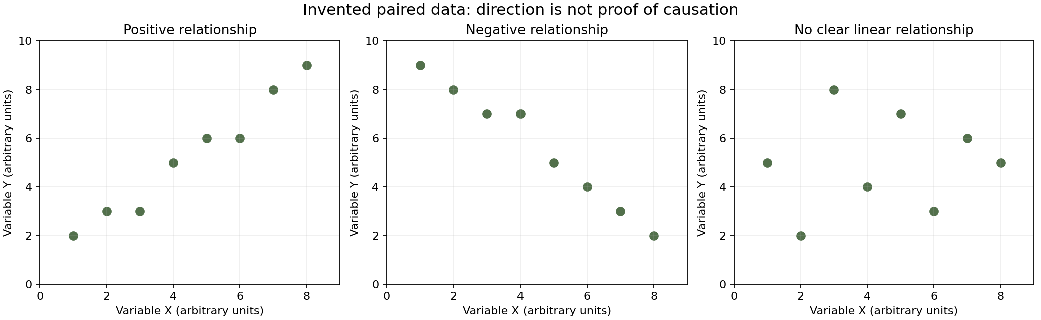
The quick answer is that a scatter plot displays paired quantitative observations. An upward overall pattern suggests positive association, a downward one suggests negative association, and a cloud with no clear linear direction suggests weak or absent linear association. Even a strong pattern does not, by itself, establish causation.
Article contents
- Quick answer: paired data are the important starting point
- Why a Bukit Timah context is not a Bukit Timah statistic
- A scatter plot differs from a bar chart
- Worked example 1: plot the six invented observations
- Paired information cannot be reconstructed from separate averages
- What a positive correlation actually describes
- A negative correlation points in the opposite direction
- No clear straight-line correlation does not mean no relationship
- Worked example 2: a U-shape fools a linear summary
- Correlation is about association, not an explanation of cause
- A confounder may affect both recorded variables
- Reverse causation is another possible explanation
- A selected group may not represent all learners
- Worked example 3: two groups hide a different pattern
- Why comparing different quizzes as if they were identical is unsafe
- Worked example 4: calculate the pooled trend’s direction
- Outliers can strongly influence a fitted line
- Worked example 5: an unusual point is not automatically an error
- The line of best fit is a summary, not a path joining every dot
- Least squares minimises squared vertical residuals
- Worked example 6: the fitted line for our six pairs
- The slope’s unit matters
- Worked example 7: make a prediction inside the observed range
- Why the intercept may not have a practical interpretation
- Interpolation and extrapolation are different
- Worked example 8: a deliberately absurd extrapolation
- Correlation strength and slope are different quantities
- Worked example 9: switching minutes to hours
- Pearson’s r is bounded between minus one and one
- Worked example 10: a perfect positive line
- r-squared should not be treated as a causality score
- A nonlinear pattern can have a high predictive structure without high r
- Measurement quality matters before trend calculation
- A missing data point is not a zero
- Repeated observations from one learner are not six independent pupils
- A before-and-after comparison does not automatically identify cause
- What a better evaluation design would ask
- Worked example 11: the importance of a comparison group
- A scatter plot can have strong association and a poor causal story
- Distinguish a model, an observation and a recommendation
- Reporting should show the axes and the observation count
- Primary preparation: read pairs without causal claims
- Lower Secondary: distinguish trend from every-point behaviour
- Upper-secondary enrichment: regression and causal caution
- Three errors tutors can diagnose independently
- A twenty-minute diagnostic with answers
- A seven-day practice sequence for better judgement
- Practice questions and checked answers
- Frequently asked questions
- Sources and connected Bukit Timah Mathematics learning

Quick answer: paired data are the important starting point
Imagine six fictional learners who all sit the same invented quiz out of 100 points. Their practice times in minutes are 10,20,30,40,50 and 60; the corresponding scores are 42,52,49,67,66 and 75.
Each time is paired with one score for the same invented learner. The six points are (10,42), (20,52), (30,49), (40,67), (50,66) and (60,75).
The overall pattern rises as practice time increases, but the score does not rise at every individual step. The learner with 30 minutes scored lower than the learner with 20. The scatter plot communicates both the general association and the variation around it.
Why a Bukit Timah context is not a Bukit Timah statistic
Families near Beauty World, Sixth Avenue and King Albert Park may naturally discuss lesson time and assessment results. That familiarity makes the question relevant to parents, but it does not justify making up actual neighbourhood achievement rates.
The six records in this article are created to produce a useful example of a positive association with non-perfect variation. They are not survey data, a tutoring case study or evidence that any real intervention caused an improvement.
A trustworthy educational explanation distinguishes the mathematical model from factual observations. The calculated line of best fit can be exactly correct for the invented coordinates without proving anything about actual students.
A scatter plot differs from a bar chart
A bar chart usually compares quantities across categories or displays frequencies. A scatter plot places a pair of numerical values at one point so that their relationship can be inspected.
Here horizontal position x represents practice minutes and vertical position y represents quiz points. A point at (30,49) means one imaginary learner practised for 30 minutes and scored 49 on the specified common quiz.
The chart should not draw a line joining points in the order learners happened to appear in a list. Connecting unrelated students with a continuous path could falsely suggest a journey through time.
Worked example 1: plot the six invented observations
Draw horizontal x marks from 0 to 70 minutes and vertical y marks from 0 to 100 quiz points. Place dots at the six stated pairs.
Look first for direction. The leftmost dot has score 42 and the rightmost score 75; many intermediate dots are also higher as x grows. But the points are not exactly aligned.
This is a positive overall relationship in the invented data. It is not proof of a deterministic rule that every additional ten minutes creates exactly a specified number of marks.
Paired information cannot be reconstructed from separate averages
Suppose a teacher records only the mean practice time and the mean quiz score without keeping which learner produced which pair. Those two summaries cannot reconstruct the scatter plot.
For our fictional table, the mean practice time is (10+20+30+40+50+60)/6 = 35 minutes. The mean quiz score is (42+52+49+67+66+75)/6 = 351/6 = 58.5 points.
Many different pairings could share the same two means while showing different associations. Correlation depends on which x goes with which y, not merely on separate summary averages.
What a positive correlation actually describes
Positive correlation means that larger x-values tend to occur with larger y-values in a broadly linear pattern. It does not require every consecutive observation to increase.
Our invented x=20,y=52 and x=30,y=49 points show a local decrease amid the overall upward tendency. A student who declares “no positive correlation because one point went down” misunderstands the concept.
The question is about the pattern of all pairs, not a rule demanding that every pair of ordered neighbours be strictly increasing.
A negative correlation points in the opposite direction
Consider another fictional chart where x is minutes of waiting and y is the number of service opportunities remaining before a cutoff. In a deliberately simple model, larger waiting times correspond to fewer remaining opportunities.
The plotted points could slope downward from left to right. This indicates negative association between the defined variables, not “bad data” or an inherently harmful mathematical relationship.
The sign of correlation describes direction only. Whether a change is desirable depends on what the axes measure and the purpose of the question.
No clear straight-line correlation does not mean no relationship
Imagine pairs generated by y=x² for x values −2,−1,0,1,2. The points form a U-shaped curve with outputs 4,1,0,1,4.
They have a strong deterministic nonlinear relationship, but the overall straight-line trend is not the right summary. A Pearson correlation coefficient can be zero for these symmetric points even though y is fully determined by x.
The lesson is to inspect the scatter plot before reducing the relationship to one number. A low linear correlation does not prove that the variables are unrelated in every sense.
Worked example 2: a U-shape fools a linear summary
For the five points (−2,4), (−1,1), (0,0), (1,1) and (2,4), the x-values balance around zero. The high y-values occur at both negative and positive x.
A horizontal line may look like a reasonable linear summary, yet it misses the U-shape. The correct generating function is y=x².
This mathematical counterexample establishes that “no positive or negative linear trend” differs from “no structure at all.” It is a useful bridge between scatter plots and quadratic graphs.
Correlation is about association, not an explanation of cause
Suppose practice time and quiz score have a positive association in a group of observed pupils. Several explanations could fit: practice might help, pupils with stronger starting knowledge might practise differently, or another factor might influence both.
The observations alone do not distinguish all those possibilities. A cause-and-effect conclusion needs a research design and evidence ruling out relevant alternatives.
This is the central statistical caution explained in Penn State’s Statistics 100 lesson on relationships and causation: association does not automatically establish a causal mechanism.
A confounder may affect both recorded variables
Imagine that access to quiet study space affects both the amount of focused practice a pupil completes and quiz performance. If that relevant condition is not recorded, the practice–score association could partly reflect it.
Other possible factors include baseline subject knowledge, prior exposure to the tested topic, question difficulty, sleep and the quality of practice. These are possible modelling considerations, not measured facts about Bukit Timah students.
The response should be to think carefully about design and measurement, not to claim that a chosen confounder definitely caused the fictional pattern.
Reverse causation is another possible explanation
A pupil who finds Mathematics difficult might spend more time practising because the material remains challenging. That could create an observed association between longer practice and lower scores.
It would be mistaken to conclude from that pattern alone that practice makes performance worse. The difficulty may influence the chosen practice duration, reversing the proposed causal direction.
The same data can support different stories unless the underlying process is investigated. Ask what causes people to receive different x-values rather than treating x as if it had been randomly assigned.
A selected group may not represent all learners
Our fictional six-person log is not a random sample of any real population. It may be useful for teaching how to draw and interpret a scatter plot, but it cannot establish a neighbourhood-wide average or effect.
Even a real dataset from one class would have a defined sampling frame. It might not represent all students in Singapore, all Secondary levels or pupils who take different courses.
The population described in a conclusion must match the evidence actually collected. “In these six invented records” is valid; “all Bukit Timah pupils improve at this rate” is unsupported.
Worked example 3: two groups hide a different pattern
Consider a separate invented illustration with two assessment groups. Group A, taking an easier quiz, has pairs (20,70) and (30,80). Group B, taking a harder quiz, has pairs (40,45) and (50,55).
Within A, more practice time accompanies a higher score. Within B, more practice time also accompanies a higher score. Yet when all four points are pooled, the broader arrangement can show a downward trend because the quiz conditions differ.
This is a simplified example of how grouping changes interpretation. It is not a claim of a causal practice effect within either group.
Why comparing different quizzes as if they were identical is unsafe
The previous four points involve two different tests. A score of 80 on one test is not automatically comparable to 55 on a harder test as a direct measurement of the same underlying ability.
A pooled scatter plot without indicating the groups may suggest the wrong narrative. Colouring points by assessment group or analysing comparable assessments separately can reveal the hidden structure.
This phenomenon illustrates a general danger of aggregation: a relationship observed within subgroups may differ from a relationship in the combined data.
Worked example 4: calculate the pooled trend’s direction
The combined fictional pairs are (20,70), (30,80), (40,45), (50,55). Their mean practice time is 35 and mean quiz score is 62.5.
The products of deviations (x−35)(y−62.5) add to a negative value: (−15)(7.5)+(−5)(17.5)+(5)(−17.5)+(15)(−7.5)=−400.
That negative covariance numerator indicates a downward pooled linear association, despite each two-point subgroup rising. The calculation shows why subgroup structure matters.
Outliers can strongly influence a fitted line
Suppose most fictional points cluster between ten and sixty practice minutes, but one extra point appears at x=120 with an unexpectedly low score. That observation could change a fitted line’s slope substantially.
It could be valid, a different measurement condition or a data-entry problem. The correct response is to inspect its source and impact rather than delete it for looking inconvenient.
Penn State’s Statistics 200 lesson notes that Pearson correlation is sensitive to outliers. A graph should be examined before reporting a correlation coefficient alone.
Worked example 5: an unusual point is not automatically an error
Imagine the original six fictional pairs plus (120,55). The new seventh point is far to the right but has a score below several shorter-practice observations.
The association of the enlarged dataset may differ from that of the first six points. We should recompute or re-examine the scatter plot rather than assume the original upward summary still applies unchanged.
If the seventh observation is genuine and comparable, it belongs in the analysis. If its 120 minutes arose from a confirmed transcription mistake, a documented correction is appropriate.
The line of best fit is a summary, not a path joining every dot
A straight line can be fitted to paired data to represent the overall linear tendency. It typically passes near the scatter, not through every point.
Individual observations can lie above or below it. The vertical differences from their fitted values are called residuals.
Drawing a zigzag line through all the dots in their listed order answers a different question and can imply changes from one learner to the next where no timeline was involved.
Least squares minimises squared vertical residuals
In simple linear regression, a line y=a+bx is commonly selected to minimise the sum of squared vertical differences between observed y-values and predicted y-values at the recorded x-values.
The squaring prevents positive and negative residuals from cancelling and gives larger deviations greater weight. The method depends on the chosen model and treats the vertical variable as the response.
This is an upper-level extension for students ready for data analysis. Primary and younger Secondary learners can begin by drawing a reasonable trend line and reading values with appropriate caution.
Worked example 6: the fitted line for our six pairs
For our invented six-point dataset, the average x is 35 and average y is 58.5. The sum of squared x deviations is 1750, and the sum of cross-deviation products is 1125.
The least-squares slope is b=1125/1750=9/14≈0.643 quiz points per additional recorded minute. The intercept is a=58.5−(9/14)×35=36.
Thus a fitted line is predicted score ≈ 36+0.643×practice minutes. This is a descriptive equation for the invented records, not a forecast of actual learning gains or a causal response to changing practice time.
The slope’s unit matters
The fitted slope of approximately 0.643 has units of quiz points per minute, because vertical changes are measured in points and horizontal changes in minutes.
It does not mean the student gains 0.643 points for each extra minute. It describes an association along the fitted line across these six hypothetical observations.
The distinction between a change in fitted prediction and a genuine treatment effect is essential. A unit can be correct while an implied causal interpretation remains unsupported.
Worked example 7: make a prediction inside the observed range
At x=40 minutes, the model predicts y≈36+(9/14)×40≈61.71 points. The actual invented observation at x=40 was 67.
The residual is observed minus predicted, so 67−61.71≈+5.29 points. This indicates the dot lies above the fitted line at that x.
A residual is not necessarily a student’s “unearned marks” or a measurement of effort. It is simply a numerical difference within the descriptive regression model.
Why the intercept may not have a practical interpretation
The fitted line predicts 36 points when x=0. But the invented dataset contains no observation at zero minutes; its practice times range from ten to sixty minutes.
It would be unjustified to claim that a student who practises zero minutes will score exactly 36, or that a score of 36 is guaranteed without preparation.
An intercept can be mathematically necessary to describe a fitted line while lying outside the observed input range. Interpret it cautiously.
Interpolation and extrapolation are different
Predicting at 35 minutes uses an x-value inside the fictional observed range [10,60]. That is interpolation within the data range, although the prediction still has uncertainty.
Predicting at 200 minutes extends far beyond the observed range. That is extrapolation and carries additional risk because the relationship may change, saturate or be invalid outside the original conditions.
A line on a screen can be extended indefinitely with a ruler. Evidence about real learners cannot.
Worked example 8: a deliberately absurd extrapolation
The invented fitted equation predicts y≈36+0.643×200≈164.6 points when x=200. But the quiz score is defined on a scale from zero to 100.
The prediction violates the response’s allowed range. That is not proof our earlier least-squares arithmetic was wrong; it is proof that extrapolating the line to 200 minutes is unsuitable.
A good student checks model domain and possible output values before accepting a numerical forecast.
Correlation strength and slope are different quantities
The slope tells how much the fitted response changes per unit x. Correlation describes the strength and direction of the linear association on a standardised scale.
Changing practice units from minutes to hours multiplies the numerical slope by sixty, but does not change the underlying Pearson correlation coefficient for the same data.
This distinction matters because a numerically steep slope is not automatically evidence of a strong correlation. Axis units can make slopes numerically larger or smaller without changing how closely points lie near a line.
Worked example 9: switching minutes to hours
Our line has slope about 0.643 points per minute. One hour contains sixty minutes, so the corresponding numerical slope in points per hour is approximately 0.643×60≈38.57.
That bigger numerical slope describes the same relationship in different x-units. It does not mean the correlation has become stronger.
Check by taking a ten-minute difference: about 6.43 points in fitted score. Ten minutes is one-sixth of an hour, so 38.57×(1/6)≈6.43 also.
Pearson’s r is bounded between minus one and one
For paired numerical data with nonzero variation in both variables, Pearson’s correlation coefficient r lies between −1 and +1. Values near +1 describe strong positive linear alignment; values near −1 describe strong negative alignment.
Values near zero indicate little linear association, not necessarily no nonlinear relationship. Undefined cases, such as one variable remaining constant, must be handled separately rather than assigned an automatic r of zero.
Our fictional six pairs have a Pearson r of approximately +0.948, a strong positive linear association in those invented coordinates. No inferential claim about real pupils follows.
Worked example 10: a perfect positive line
Imagine points (1,2), (2,4), (3,6) and (4,8), all lying exactly on y=2x. Their Pearson r is +1 because they follow a perfectly increasing straight line with nonzero variation.
A different set (1,8), (2,6), (3,4), (4,2) lies exactly on y=10−2x and has r=−1.
These mathematical datasets demonstrate what the extreme correlation values mean geometrically. Neither one asserts a causal mechanism between x and y.
r-squared should not be treated as a causality score
The square of the sample correlation, r², describes the proportion of sample response variation accounted for by a least-squares linear model with an intercept under the usual simple-regression setup.
For the fictional r≈0.948, r² is about 0.898. It would be wrong to say “90% of the pupil’s success was caused by practice” from that value.
Model fit and causal explanation are not the same. Penn State’s regression guidance cautions against treating a strong statistical relationship as a cause-and-effect proof.
A nonlinear pattern can have a high predictive structure without high r
Return to the U-shaped data y=x² with x symmetrical around zero. The response is exactly known from x, but its linear correlation can be zero.
This is not a contradiction. Pearson r measures linear direction and alignment, while a quadratic relationship bends.
A graph inspection should precede a correlation summary. Students should never replace the actual shape of the scatter with a single r-value without considering whether the linear model fits.
Measurement quality matters before trend calculation
Suppose some fictional practice minutes were reported from memory and others were timed precisely. Their reliability differs. A learner may also define “practice” inconsistently, sometimes including breaks or passive video viewing.
Comparing those numbers as though they represent the same quantity can create a misleading association even when the graph is computed correctly.
For a meaningful analysis, define start and stop rules, ensure the quiz score is comparable and decide how missing or interrupted sessions are recorded.
A missing data point is not a zero
If one fictional learner did not report practice time, the x-coordinate is missing. It should not automatically be entered as zero minutes.
Zero is a positive claim that the learner completed no time under the definition. Missing means the observation is unknown or unrecorded.
Substituting zero for missing values can alter averages, slopes and correlations. The correction requires inspecting the data collection procedure, not merely adding another dot.
Repeated observations from one learner are not six independent pupils
A scatter plot of six daily pairs from one student may show a different structure from six pairs collected from six different students. There may be time trends, learning carryover or repeated-measure dependence.
The source of each pair should therefore be documented. Treating repeated daily measurements as independent observations can exaggerate how much independent information a dataset contains.
This is an upper-level caution. Younger learners can begin by specifying what each dot represents: a pupil, a session, a day or another observational unit.
A before-and-after comparison does not automatically identify cause
Suppose a learner studies a topic, then obtains a higher quiz mark the following week. That observed improvement may be meaningful, but the second quiz could differ in difficulty or the learner could have benefited from ordinary classroom teaching.
A credible progress assessment uses comparable tasks, documents the intervention and considers other plausible influences. Even then, causal conclusions may remain uncertain without a stronger study design.
A tutor can use scores to target weaknesses without promising a measured causal effect unsupported by the evidence.
What a better evaluation design would ask
To investigate whether a particular learning intervention improves performance, a study would need clear outcome measures, suitable comparison groups and a way to address baseline differences and confounding.
Random allocation can improve causal identification in appropriate research settings, but it requires ethical, practical and methodological safeguards. A small classroom log by itself does not become a trial.
Parents should ask for evidence of changing independent work, better transfer to unfamiliar problems and consistent school feedback, not merely a graph in which two numbers rise together.
Worked example 11: the importance of a comparison group
Imagine a purely fictional intervention group whose average quiz score rises from 60 to 70. A similar comparison group also rises from 60 to 68 over the same period.
The intervention group’s ten-point improvement does not, by itself, establish ten points of impact. The comparison group’s eight-point improvement suggests broader factors may be present.
The difference between the two changes is two points in this simplified example, but interpreting that as a causal effect still requires assumptions about comparability, trends and study design. It is a teaching illustration, not actual programme evidence.
A scatter plot can have strong association and a poor causal story
Imagine recording outdoor temperature and ice cream sales on many invented days. Both may increase together without one automatically being the sole direct cause of the other.
Temperature can influence demand, calendar conditions can affect foot traffic, and other factors may vary. The data alone do not reveal which explanations have been adequately tested.
This familiar illustration is useful because children understand that correlation invites a question rather than settles an explanation.
Distinguish a model, an observation and a recommendation
A model is a simplified relationship such as predicted score = 36+0.643×minutes for our invented dataset. An observation is an actual paired record within a defined data source. A recommendation is a decision made after considering goals and evidence.
The three should not be collapsed. The regression equation does not prescribe a fixed daily practice duration for every child, and invented observations cannot validate a programme.
A mathematically mature response names the level at which each claim is supported.
Reporting should show the axes and the observation count
A chart intended for parents should label practice in minutes, quiz score in points out of 100, and the fact that six fictional observations were used. Without these details, the apparent trend is hard to evaluate.
If the plot includes a fitted line, identify it as a fitted line rather than an established law. If the chart excludes an outlier, explain and justify the exclusion rather than hiding it.
The reader should be able to reconstruct the basic meaning of the graphic without guessing units or data selection.
Primary preparation: read pairs without causal claims
Younger pupils can begin by matching each day or learner with two recorded values in a table, then plotting simple pairs on graph paper when appropriate.
Ask “What does this dot stand for?” and “Which axis shows the minutes?” before discussing whether dots generally rise or fall.
The initial goal is graphical literacy: read a paired record accurately. Formal Pearson r and least squares belong to more advanced study.
Lower Secondary: distinguish trend from every-point behaviour
A Secondary learner can plot six points, describe positive or negative association qualitatively and notice deviations from a broad pattern.
Provide a chart in which the dots generally rise but two successive x-values have reversed y-values. The student should be able to explain why a positive association can still exist overall.
This builds a stronger interpretation skill than memorising “up is positive” without reading the actual distribution.
Upper-secondary enrichment: regression and causal caution
Students who are ready can compute means, covariance-related sums, fitted slopes, residuals and Pearson correlation, subject to their actual syllabus.
The important extension is understanding what those coefficients mean and what they do not mean. A regression slope is a modelled association; a causal effect requires appropriate design and assumptions.
If the student’s course does not require full regression calculations, qualitative scatter-plot interpretation can still be valuable enrichment without falsely claiming it is examination content.
Three errors tutors can diagnose independently
One pupil may swap x and y coordinates. Another may link scatter points in list order as if they form a journey. A third may interpret positive correlation as proof that extra practice caused improvement.
The first needs coordinate-reading repair, the second needs chart-type understanding, and the third needs statistical reasoning about alternative explanations.
A small-group teaching approach should address the earliest invalid assumption rather than presenting every error as a calculation slip.
A twenty-minute diagnostic with answers
Minutes 1–5: Plot fictional pairs (10,42), (20,52), (30,49), (40,67), (50,66), (60,75). State which variable belongs on each axis.
Minutes 6–10: Describe the overall association as positive but not perfectly linear. Find mean x=35 and mean y=58.5.
Minutes 11–15: Use fitted line y≈36+0.643x to predict at x=40. The predicted score is about 61.7; the observed fictional score was 67, giving residual about +5.3.
Minutes 16–20: Ask, “Do these six points prove that additional practice causes higher marks?” The correct answer is no; selection, baseline knowledge and other conditions remain untested.
A seven-day practice sequence for better judgement
Day one reads paired tables. Day two plots points with units. Day three distinguishes upward, downward and nonlinear patterns. Day four introduces outliers and missing observations.
Day five draws or interprets a fitted straight line. Day six discusses residuals and extrapolation. Day seven gives a new fictional dataset and asks the child to separate supported descriptive statements from unsupported causal claims.
The difficulty level should follow the learner’s prerequisites. Formal regression should never substitute for basic coordinate understanding.
Practice questions and checked answers
A. Points (1,2), (2,4), (3,6) lie on what simple line? Answer: y=2x.
B. In the six-pair invented dataset, what is mean practice time? Answer: 35 minutes.
C. Using y=36+0.643x, predict at x=20. Answer: approximately 48.9 points. This is a fitted prediction, not the actual observation of 52.
D. If one observation at x=120 is added, must the fitted slope stay unchanged? Answer: no; a distant point can substantially change the line.
E. Does a Pearson correlation near zero rule out a U-shaped relationship? Answer: no; it describes weak linear association and can coexist with a strong nonlinear pattern.
Frequently asked questions
Does positive correlation mean every new point is higher than the previous one?
No. It describes an overall positive linear tendency. Individual dots can deviate from that pattern.
Does a strong r-value prove that one variable causes the other?
No. A high linear correlation can arise through confounding, selection, reverse causation or other structures.
Is a scatter plot the same as a line graph?
No. A scatter plot displays paired observations. Connecting unrelated points in sequence may imply a false continuity.
Why is a line of best fit not expected to pass through every dot?
It summarises the overall linear association and typically leaves positive and negative residuals.
Are the six pupils in this guide actual Bukit Timah students?
No. Every record is an invented teaching example, not an actual student dataset.
Why shouldn’t we extrapolate far beyond observed practice times?
The fitted relationship may not continue outside the recorded range and may produce impossible quiz-score predictions.
Can a perfectly accurate computation still support a wrong conclusion?
Yes. The formula may be calculated correctly while the data are unrepresentative, variables are not comparable or a causal claim exceeds the design.
Is regression required for every Secondary learner?
No. Methods and assessment expectations vary by level and syllabus; full regression is an extension where appropriate.
What would demonstrate a useful improvement in data reasoning?
A learner can identify paired variables, describe a trend accurately, explain deviations and name at least one reason correlation alone cannot establish cause.
Sources and connected Bukit Timah Mathematics learning
The Penn State STAT 100 lesson on relationships, STAT 200 discussion of descriptive relationships and outliers and STAT 501 regression cautions support the distinction between association, outliers, fitted lines and causality. Their lessons do not supply the invented pupil dataset used in this article.
For Singapore school context, consult the MOE Primary Mathematics syllabus and SEAB 2027 G3 Mathematics syllabus directory. Specific advanced regression calculations should not be assumed examinable for every course.
Continue with Mathematics in Bukit Timah: how to read misleading graphs to check visual claims, or mean, median and outliers in reading-time data for univariate descriptive statistics. The immutable Clementi Secondary 1 Mathematics tutorial reference anchors the practical focus on explaining reasoning before performing a procedure quickly.
The habit to keep is identify exactly what each point measures, inspect the full pattern, test the model’s limits and never promote an observed association into a proven cause without suitable evidence.
Continue this four-article Mathematics in Bukit Timah batch: Counting grid paths, Pascal’s triangle and combinations · Quadratic graphs, arches and turning points · Coordinate distance, midpoints and bisectors. These original guides use different mathematical models, with worked questions, learning diagnostics, careful assumptions and sources.