
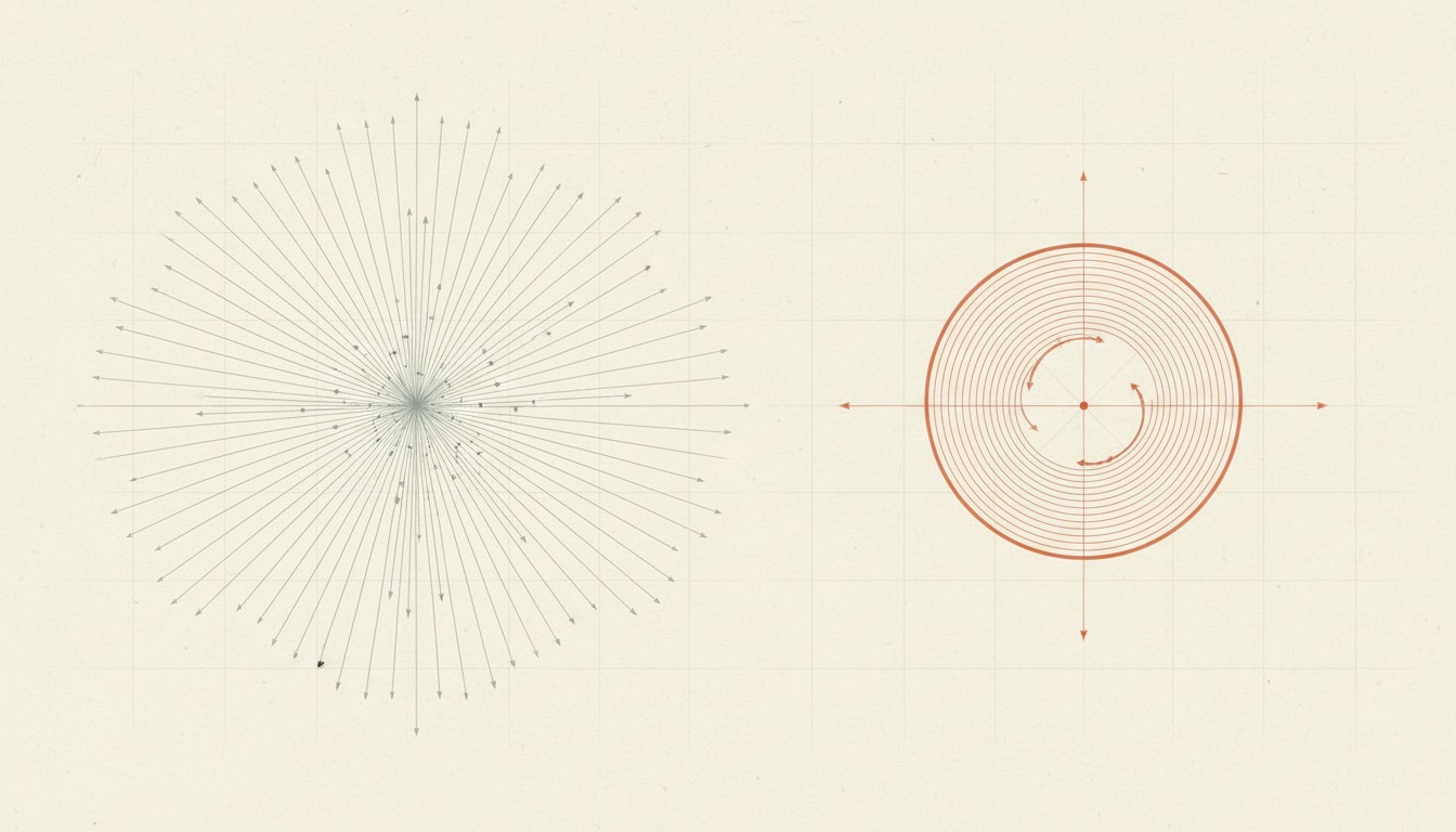
Did you know? A large matrix can sometimes be approximated without first computing all of its singular vectors. Randomized singular value decomposition (randomized SVD) uses a small random sketch to find a subspace that captures much of the matrix’s dominant structure. It then solves a much smaller deterministic decomposition inside that subspace. The result can be a useful low-rank model for dimensionality reduction, recommendations or scientific data, but it is an approximation whose error and data assumptions must be checked.
The practical algorithm is to choose a target rank and an oversampling budget, draw a suitable random test matrix, multiply the data matrix by it, orthonormalise the resulting columns, project the original data into that subspace, and compute a small SVD. Power iterations can improve separation when singular values decay slowly, at the cost of extra matrix passes and numerical considerations. Compare reconstruction error, downstream usefulness, memory and latency against the exact or otherwise appropriate baseline.
This guide provides an original hand-computable matrix example, clear dimensions and units, an explicit memory case, failure diagnoses and a changed-context exercise. All numerical examples are teaching constructions; no model training or benchmark is claimed.
Contents
- The problem: preserve dominant structure without every singular vector
- What singular values tell us—and what they do not
- Random projection finds a candidate column space
- From reduced matrix to approximate singular vectors
- Solved diagonal-matrix case: a visible imperfect sketch
- Why target rank and sketch width are different
- Power iterations emphasise directions with large singular values
- Worked memory case: what a 100,000 by 2,000 matrix costs
- Reconstruction quality is different from predictive usefulness
- Randomized SVD, PCA and TruncatedSVD are related but not identical
- Sparse matrices, streaming and matrix-pass limitations
- Numerical stability and the danger of nearly dependent columns
- Random seeds, oversampling and repeatability
- Changed-context exercise: when the neglected direction becomes essential
- Ten failure modes and their practical repairs
- Limits and ethical considerations of compression
- Frequently asked questions
- Reader pathways and original primary references
The problem: preserve dominant structure without every singular vector
Many datasets can be represented as matrices: customers by measured preferences, documents by term features, images by pixel values, or machines by sensor readings over time. When a matrix has thousands or millions of rows, its full decomposition may be unnecessary if the application needs only a small number of dominant patterns. The computational question is which patterns can be retained without distorting the task’s essential information.
Singular value decomposition writes a real matrix A as UΣVᵀ, where U and V contain orthonormal singular-vector directions and Σ contains nonnegative singular values ordered from largest to smallest. The larger singular values correspond to directions with more squared Frobenius energy in the matrix. A low-rank approximation retains only some leading components.
Exact truncated SVD can be useful, and modern algorithms need not calculate a complete dense factorisation. But dense matrices, large input dimensions or costly passes through storage may make a carefully chosen randomized range finder attractive. The algorithm leverages matrix multiplication, QR factorisation and a smaller SVD rather than promising to eliminate all linear algebra.
The goal is to approximate the action of A on important directions with a basis Q containing far fewer columns than A has rows or columns. Once those columns capture the dominant range, work can proceed with B=QᵀA, whose first dimension is small. This is a change in the size of the central decomposition problem, not a claim that all information can be kept.
The original research Finding Structure with Randomness by Halko, Martinsson and Tropp studies probabilistic algorithms for approximate matrix decompositions and the conditions under which they are accurate and efficient. Its theory and experiments motivate the approach; the actual benefits depend on the matrix and implementation.
What singular values tell us—and what they do not
The squared Frobenius norm of a real matrix is the sum of the squares of all its entries. It is also the sum of squared singular values. If a matrix has singular values five, two and one, the total squared Frobenius energy is 5²+2²+1²=25+4+1=30, in squared units of the original matrix entries.
Keeping the largest singular value in an ideal rank-one truncated SVD preserves 25/30 of this squared energy, or about 83.333%. Keeping the two largest preserves (25+4)/30=29/30≈96.667%. Energy retention is a geometric reconstruction statement, not a claim that a classifier or recommendation engine will perform with the same percentages.
The Eckart–Young–Mirsky theorem tells us that truncated SVD is the best rank-k approximation under familiar unitarily invariant norms, including the Frobenius norm, under the theorem’s conditions. But the optimal reconstruction is still an approximation when neglected singular values are nonzero. The residual can matter enormously if a small singular direction carries a rare but important signal.
A singular-value spectrum that falls rapidly suggests there may be a compact low-rank description. A flat or slowly decaying spectrum makes approximation more difficult at a small rank. Power iterations can help isolate dominant directions but add work. Model selection should be driven by the task, not simply by a desire for a very low rank.
Rescaling rows or columns changes the spectrum. Data preprocessing, missing-value patterns and the meaning of numerical units influence which directions appear dominant. Before celebrating the leading singular vectors, make sure their geometry corresponds to the question the application needs to answer.
Random projection finds a candidate column space
Choose a target rank k and an oversampling parameter p, giving a sketch width l=k+p. Generate a random matrix Ω with shape n×l for a data matrix A with shape m×n. A common choice is standard Gaussian entries, though other sketch distributions exist. Then compute Y=AΩ, which has shape m×l.
The columns of Y are combinations of A’s columns. Because random test vectors generally touch many directions, Y can reveal much of the dominant column space even though its width l is small relative to n. This is a probabilistic statement under suitable assumptions, not a deterministic guarantee for every draw.
Next orthonormalise the columns of Y, usually through a numerically stable QR factorisation, obtaining Q with orthonormal columns. The matrix QQᵀ acts as a projector onto the chosen subspace. The approximation QQᵀA keeps the portion of A that lies in that subspace and discards what lies orthogonal to it.
That discarded component is the range-finder error. A direct diagnostic is a norm of A−QQᵀA, where the norm should be stated explicitly. Computing a full exact residual for a huge dataset may itself be expensive, so a practical implementation can use carefully designed estimates or sampled checks, with their uncertainty labelled.
Once Q is available, compute B=QᵀA. This reduced matrix has l rows and n columns. Its shape captures the computational advantage: the subsequent decomposition is performed in a lower-dimensional representation rather than on the entire original m×n matrix.
From reduced matrix to approximate singular vectors
Compute an SVD of the smaller B: B=U_BΣVᵀ. Map the left singular vectors back to the original row space using U≈QU_B. If only k components are needed, retain the leading k columns and singular values. This gives an approximate rank-k factorisation A≈U_kΣ_kV_kᵀ.
The procedure combines randomness and determinism in different places. Randomness chooses a candidate subspace; the smaller SVD then finds the best directions within that chosen subspace. Calling the entire result random guessing obscures the careful numerical structure of the algorithm.
The approximation can fail if Q misses an important direction. The small SVD can be perfectly computed and still cannot recover information already excluded from Q’s column space. That is why oversampling, power iterations and residual checks belong to the design.
Keep dimensions clear. If A has 100,000 rows and 2,000 columns, k=20 and p=10, then Ω has shape 2,000×30, Y and Q have shape 100,000×30, and B has shape 30×2,000. The final retained U_k has shape 100,000×20, Σ_k has 20 diagonal entries, and V_kᵀ has shape 20×2,000.
Numerical implementations may use different conventions, data types or orientation choices, and may transpose a wide matrix to optimise work. A reviewer should inspect actual array shapes and reconstruction, not infer correctness solely from the function name.
Solved diagonal-matrix case: a visible imperfect sketch
Use a fully invented 3×3 diagonal matrix A=diag(5,2,1). Its exact singular values are five, two and one, with total squared Frobenius norm 25+4+1=30. The best rank-one approximation keeps the first diagonal entry and discards the others. Its squared Frobenius residual is 2²+1²=5, so the residual norm is sqrt(5)≈2.236.
Now choose a deliberately fixed one-column sketch Ω=(1,1,0)ᵀ. This is not claimed to be a Gaussian sample; it is selected to make the projection arithmetic transparent. Multiplication gives Y=AΩ=(5,2,0)ᵀ. Its norm is sqrt(29), so the normalised Q is (5,2,0)ᵀ/sqrt(29).
Project A into this subspace: B=QᵀA=(25,4,0)/sqrt(29). Since B is a row vector, its squared Frobenius norm is (25²+4²)/29=(625+16)/29=641/29≈22.103448. The original matrix’s squared norm is 30, so the projector’s squared residual is 30−641/29=229/29≈7.896552.
The randomized rank-one sketch therefore has residual norm sqrt(229/29)≈2.810, worse than the best rank-one residual sqrt(5)≈2.236. It preserves (641/29)/30=641/870≈73.678% of squared energy, less than the optimal 83.333%. This is a truthful small example of approximation error, not a demonstration that randomized SVD is usually poor.
The lesson is that the small SVD cannot recover a dominant direction the sampled subspace represents imperfectly. More or better selected sketch directions, oversampling and suitable power iterations can improve the result, but they must be evaluated with real error checks.
Why target rank and sketch width are different
The desired output rank k may be twenty, while the sketch width l is thirty because ten additional directions are sampled. This oversampling gives the randomized range finder room to capture important singular directions even when one random draw represents them poorly. The extra components can be discarded after the smaller SVD chooses the best k directions within the sketched space.
Oversampling is not an unlimited fix. Larger l increases intermediate matrix width, projection time and memory. At some point an approximation that uses too many extra vectors loses the computational advantage that motivated it. A suitable value depends on spectrum, error tolerance, software defaults and resource constraints.
An application’s target k should follow a real requirement. Keeping twenty components because a tutorial uses that number is not a principled design. If downstream reconstruction, ranking or prediction worsens sharply below forty, the right target may be larger. If ten components already meet the requirement, retaining more may be unnecessary.
Record both k and p. A report saying ‘we used rank twenty’ without mentioning an oversampled sketch width of thirty hides part of the computational cost. It also makes replication harder when two libraries use different default oversampling behaviour.
Where accuracy matters, compare several combinations of rank and oversampling on data that reflect deployment. A method may improve the Frobenius reconstruction but not downstream recall, because those are different objectives.
Power iterations emphasise directions with large singular values
When singular values decay slowly, a basic random sketch may not separate leading directions well. Power iteration can strengthen dominant components before orthonormalisation. In a conceptual form, apply Y=(AAᵀ)^q AΩ for a nonnegative integer q, using numerically stable matrix multiplications and intermediate orthonormalisation rather than forming enormous products explicitly.
Return to the toy A=diag(5,2,1) with Ω=(1,1,0). Without a power step, Y=(5,2,0), whose first-to-second coordinate ratio is 5/2=2.5. With one conceptual power iteration, Y=(AAᵀ)AΩ=(125,8,0); the ratio becomes 125/8=15.625. The sketch points much more strongly toward the dominant first singular direction.
The larger separation improves potential approximation of the leading component in this toy case. It also costs extra passes and multiplications and may amplify numerical conditioning issues. Stable implementations include normalisation procedures to avoid losing useful directions to rounding error. Do not compute the full AAᵀ matrix for a massive dataset merely because it appears in the mathematical expression.
The official scikit-learn randomized_svd documentation describes n_iter and power_iteration_normalizer among its controls. Inspect the exact library version and matrix shape before copying values from an example, since defaults and recommended settings depend on software and target use.
More iterations are not automatically better. They increase work, and an unstable implementation or inappropriate data may still produce misleading results. Use an error budget and runtime measurements to choose a modest number of iterations rather than treating q as a prestige parameter.
Worked memory case: what a 100,000 by 2,000 matrix costs
Imagine an invented dense A with 100,000 rows and 2,000 columns. It contains 200,000,000 entries. At four bytes each in float32, raw storage is 800,000,000 bytes, or 800 MB in decimal units. A full economy-size left singular-vector matrix with 2,000 columns would be comparably large before considering other decomposition storage and workspace.
Suppose we need k=20 components and choose p=10, so l=30. The sketch Y has 100,000×30=3,000,000 entries, or 12 MB at four bytes each. The reduced B has 30×2,000=60,000 entries, or 240,000 bytes, or 0.24 MB. These sizes reveal why the sketch and reduced matrix can be smaller than a full factor.
However, the original A still occupies 800 MB if stored in memory, and QR factors, model outputs, temporary arrays and solver workspaces add overhead. The reduced B might need a different precision or layout. Reading data from disk, multiplying A by Ω and performing power iterations can dominate runtime.
The ratio between the displayed sketch Y and A is 12/800=0.015, or 1.5%. That is the ratio of two specified raw arrays, not a promise of 98.5% total memory savings. If an implementation streams A rather than loading it whole, its memory story is different again.
An honest resource comparison reports the stored input representation, number of passes, peak process memory and actual elapsed time. A theoretically small sketch can still be inefficient on badly chosen hardware or under a costly repeated-pass schedule.
Reconstruction quality is different from predictive usefulness
Randomized SVD can be evaluated through matrix reconstruction error, such as ||A−U_kΣ_kV_kᵀ||_F. That tells us how well the retained low-rank components reproduce entries of A under the selected norm. It does not automatically tell us whether a classifier trained on those components correctly identifies rare events or whether a recommendation system treats users fairly.
Suppose a matrix has a huge common pattern and a small but important anomaly. A rank-k approximation minimising global squared reconstruction error may ignore the anomaly because it contributes little to total energy. If the application is fraud detection or safety monitoring, that neglected direction could be the very signal the reader cares about.
Validate the downstream task separately. A document matrix may be decomposed for search; the relevant measures could include retrieval recall or ranking quality. A sensor matrix may be compressed; the relevant measures could include reconstruction of important failure states. Preserve a distinct held-out evaluation and do not choose k merely from in-sample reconstruction.
Also consider data leakage. If a decomposition is fitted on the complete dataset before splitting train and test records, later model evaluation may incorporate information from held-out cases. Where the intended deployment learns from training data only, fit the decomposition inside the training pipeline and transform test data with the retained factors.
One useful report shows both residual reconstruction error and the end-user outcome measure, along with rank, sketch width, power iterations and random seed. This is far more informative than saying ‘the embedding has high explained variance’ without defining what variance means.
Randomized SVD, PCA and TruncatedSVD are related but not identical
Principal Component Analysis is often implemented through a singular value decomposition of a centred data matrix. Centring subtracts feature means so the decomposition describes directions of variation around the mean. TruncatedSVD on an uncentred matrix instead captures dominant singular directions of the original entries and can be useful for sparse text data where centring would destroy sparsity.
Randomized SVD is a computational algorithm used to approximate dominant singular directions. It does not by itself prescribe centring, standardisation, missing-value handling or an application-specific objective. A library may use randomized SVD internally for PCA or TruncatedSVD, but the statistical meaning depends on the surrounding preprocessing.
Imagine a feature column with all values close to a large constant. Without centring, that mean level can dominate the leading singular vector. After centring, the analysis instead focuses on deviations. Neither is automatically right; a document term matrix and a physical measurement table may demand different treatments.
When fitting PCA for downstream prediction, estimate feature means on the training set and apply those same means at inference. If a sparse representation would become dense through centring, select an algorithm and model interpretation that respect the memory constraints. Do not silently describe uncentred TruncatedSVD components as ordinary centred principal components.
The best reference point is the actual estimator’s documentation and the matrix supplied to it. A correct randomized algebraic routine can still answer a different statistical question from the one the project owner intended.
Sparse matrices, streaming and matrix-pass limitations
Many document-term matrices contain mostly zero entries. A sparse representation can preserve that structure and make matrix multiplication cheaper than using a full dense array. Randomized algorithms can often exploit efficient sparse multiplications, but intermediate sketches or power-iteration arrays may still become dense. Peak memory must account for both formats.
One major engineering cost is the number of times a dataset is read. For an on-disk or remote matrix, each pass may incur substantial I/O. Power iterations improve subspace quality in some conditions but require additional applications of A and Aᵀ. When data access is expensive, a lower-pass method with somewhat higher approximation error may be preferable.
Streaming implementations need careful treatment of row order, shapes, data versions and failure recovery. If a dataset changes between passes, the mathematical assumption that every multiplication uses the same A can fail. Keep a stable snapshot or version identifier when exact consistency matters.
Distributed execution adds another constraint: QR orthonormalisation and aggregation must maintain numerical stability and correct column alignment. A crash halfway through assembling a sketch may leave an apparently plausible but incomplete matrix. Verify row counts, expected dimensions and input checksums before decomposing.
Do not treat a published asymptotic complexity as a guaranteed end-to-end speedup. Real performance depends on matrix sparsity, memory bandwidth, parallel hardware, implementation choices and the tolerated approximation error.
Numerical stability and the danger of nearly dependent columns
When Y’s columns are nearly linearly dependent, its QR factorisation becomes sensitive to floating-point and rank-deficiency issues. A stable routine should detect effective rank and produce a sensible orthonormal basis. If l exceeds the numerical rank of A, some sampled directions may add little or no useful information.
Power iteration can magnify dominant singular values relative to smaller ones. That is its benefit and also a numerical risk: weak directions can become harder to represent in finite precision. Stable algorithms often alternate multiplications with orthonormalisation or normalisation steps to maintain useful numerical scale.
Do not form (AAᵀ)^q as a huge explicit matrix power. The formula is conceptual; practical routines apply A and Aᵀ successively and use stable orthogonalisation. Explicitly forming enormous dense products can erase the algorithm’s memory advantage and worsen numerical behaviour.
Singular vectors also have sign ambiguity: multiplying a singular vector by −1 while compensating in its paired factor preserves the reconstructed matrix. Two correct runs may report sign-flipped component coordinates. Compare reconstructed subspaces or invariant quantities rather than treating a harmless sign change as a model failure.
Reconstruction error and orthogonality checks are concrete. Verify QᵀQ is close to the identity within an appropriate numerical tolerance and compare the approximate reconstruction against accessible exact or independently estimated benchmarks. The tolerance depends on precision, conditioning and use.
Random seeds, oversampling and repeatability
A fixed random seed can make Ω reproducible, which is useful for investigating a reported result. But one lucky seed may yield a better subspace than another. Small oversampling and difficult spectral structure can increase run-to-run variability. Repeated sketches or error bounds can help characterise that sensitivity.
Do not promote an algorithm as reliable because one seed produced an attractive chart. Record the distribution or range of relevant held-out results across appropriate repetitions, especially when decisions depend on small changes in retrieval or classification performance. Keep all the unsuccessful trials in the analysis, not only the best run.
Random seed control is distinct from data version control. If row order, preprocessing, numerical precision or input content change, the same seed does not recreate the same experiment. Save enough configuration and data identity to reproduce the matrix actually decomposed.
Different libraries may use different random number generators, oversampling defaults or sign conventions. Reproducing exact floating-point values across versions is not always realistic. Reproducing the mathematical validity and task-quality conclusion is more important than insisting that every singular vector’s printed sign match.
An agent preparing a report should be explicit about what was executed. A formula and a toy matrix are teaching material; a claim of measured approximation quality requires an actual run, stored result and repeatable procedure.
Changed-context exercise: when the neglected direction becomes essential
Return to the invented matrix A=diag(5,2,1). A best rank-one approximation keeps the singular value five and drops the directions associated with two and one. Its Frobenius residual norm is sqrt(5)≈2.236. Now imagine the third coordinate encodes a rare but decisive safety signal rather than unimportant background variation.
The best rank-one reconstruction still minimises global Frobenius error, but it erases that third coordinate. A system that uses only the retained component may miss the safety information entirely. Better numerical reconstruction of large common entries is not a guarantee of suitability for the changed task.
Suppose the application’s goal changes from overall image compression to detecting that rare safety signal. The correct choice may require retaining a targeted feature, changing the loss, increasing rank or avoiding low-rank compression for that decision. The decomposition did not become mathematically incorrect; the application’s success criterion changed.
Now consider a related numerical change: A=diag(5,4,3) has squared singular-value energy 25+16+9=50. Keeping only the largest value retains 25/50=50% of squared energy, far less than the 83.333% in the earlier matrix. The same rank choice behaves differently because the singular-value spectrum is flatter.
This transfer question has two answers: mathematical approximation quality depends on spectral decay, and user-level relevance depends on which information the task needs. Robust intelligence checks both before declaring the compression successful.
Ten failure modes and their practical repairs
Failure one is treating the requested output rank as the whole sketch width. Repair by documenting k, oversampling p and actual l=k+p. Failure two is transposing the wrong dimensions so Ω has an incompatible shape. Repair with matrix-shape assertions before large multiplications.
Failure three is assuming one random draw always captures the dominant range. Repair by checking approximation error and considering oversampling or repeated seeds. Failure four is making power iteration unstable by forming huge explicit products or skipping needed normalisation. Repair by using a well-tested stable implementation and profiling passes.
Failure five is reporting low reconstruction error as proof of good prediction. Repair by evaluating the intended downstream metric, including rare-important cases. Failure six is performing PCA-like analysis without understanding whether the matrix was centred. Repair by documenting preprocessing and estimator semantics.
Failure seven is fitting a decomposition on final test data and then reporting a downstream model’s performance as independent. Repair by fitting transformations only within the permitted training split. Failure eight is comparing dense arrays without counting sparse formats, intermediate workspaces and data-loading costs. Repair with measured peak memory.
Failure nine is treating harmless sign flips of singular vectors as evidence that a decomposition is wrong. Repair by comparing subspace projections and reconstruction. Failure ten is reusing a stale sketch after a dataset version changed during streaming. Repair with immutable input identities and consistent matrix passes.
A useful debugging order is: input meaning, shapes, exact small matrix, orthogonality, residual error, repeated seed stability, downstream held-out performance and actual resource usage. Each step checks a different failure surface instead of burying the problem inside an unexplained library call.
Limits and ethical considerations of compression
Randomized SVD assumes a useful low-rank structure for the chosen objective. When singular values decay slowly, a small rank may produce a poor approximation. Power iterations and oversampling can help, but cannot make genuinely high-rank information disappear without loss.
Compression can remove subtle minority or edge-case information because global squared error emphasises large common patterns. In education, medicine or safety, the most important signal may not be the largest source of variance. Preserve additional tests and human review where a missed rare event would matter.
The algorithm does not solve missing values, privacy, data rights, sample selection or causal interpretation. Those issues arise in the construction and use of the matrix. A mathematically excellent decomposition can still support a harmful or misleading decision when data are biased or authority is missing.
Performance claims must be bounded by the actual hardware and source matrix. A small sketch is not evidence of low total energy use, a fixed latency or guaranteed scalability. Time, memory and passes must be measured. Do not invent benchmark percentages from symbolic complexity alone.
Scientific studies and official library docs give a defensible starting point, not permission to claim a particular production improvement without execution. This article uses only hand-checked fictional data for its numerical teaching cases.
Frequently asked questions
What does randomized SVD do? It finds a candidate low-dimensional subspace using random matrix multiplication, then computes an SVD of a smaller projected matrix.
Is it the same as a full exact SVD? No. It approximates dominant singular components, and error depends on the sketch, rank, spectrum and numerical choices.
What is oversampling? It adds extra sketch columns beyond the requested output rank to improve the chance of capturing important directions.
Why use power iterations? They can amplify separation between dominant and weaker singular directions, but cost extra multiplications and require numerical care.
What do the singular values represent? They measure the strength of orthogonal directions in a matrix under SVD geometry, not automatically the importance of features for a supervised task.
Is randomized SVD the same as PCA? It is a computational method that can support PCA; PCA’s statistical meaning depends on centring and the data representation.
Why can a low-rank approximation miss a rare signal? Global reconstruction objectives often prioritise large common energy, whereas rare features may contribute little energy while being consequential.
Can the method work on sparse text data? Suitable implementations can exploit sparse multiplication, but intermediate arrays and centring choices must be considered.
Does fixing a seed guarantee correctness? No. It improves repeatability of one draw, not guaranteed fidelity or future generalisation.
What should be evaluated before deployment? Matrix reconstruction error, numerical stability, relevant held-out task outcomes, memory, latency and the data-shift conditions that matter.
Reader pathways and original primary references
If you are learning matrix algebra, solve the diagonal A=diag(5,2,1) case by hand, compute its best rank-one residual and the illustrative random-sketch residual, then explain why the latter is larger. Try the spectrum A=diag(5,4,3) and compare energy retention.
If you build models, document A’s shape, preprocessing, target rank, oversampling, power-iteration count, seed and estimator version. Verify orthogonality and reconstruction, then evaluate the downstream task on data not used to choose the decomposition.
If you review an AI system, ask which information the low-rank factors discard, whether rare cases matter and whether the reported efficiency includes data loading and intermediate arrays. Do not mistake a low-dimensional representation for a guarantee of fairness or safety.
Primary research: Halko, Martinsson and Tropp, Finding Structure with Randomness, also published in SIAM Review 53(2), 2011. Official implementation reference: scikit-learn randomized_svd.
Related verified live reading includes Spectral Normalization — Singular Values and Power Iteration, Product Quantization — Compressed Vectors, and the How AI Works overview. Their specialist reader problems differ from randomized low-rank matrix decomposition.