
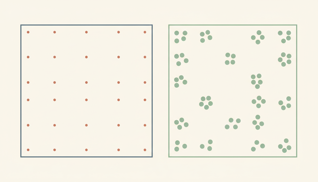
Did you know? Two rare things occurring together can feel like evidence of a strong relationship even when the relevant rates are equal. Illusory correlation is a mistaken or exaggerated perception of association. A conspicuous negative event involving a small group, an unusual software component or an unfamiliar school class may remain especially memorable, leading observers to infer a pattern that the full denominator does not support.
The practical repair is to reconstruct the complete comparison table: count both outcomes in each group, divide each group’s outcome count by its own exposure total, and inspect uncertainty and measurement conditions. Distinguish what was noticed from what was observed. A memorable combination is a reason to ask for the full data, not permission to make a judgement about a person or population.
This guide traces the primary research on distinctive co-occurrences, derives invented examples with exact denominators, considers stereotype harms and organisational incident reviews, and shows how the conclusion changes when rates—not merely event counts—change. It is about human and collective intelligence, not a deterministic rule that every observer always commits the bias.
Contents
- The real question: is there an association or only a memorable coincidence?
- What the original experiments actually investigated
- A complete four-cell table with equal rates
- Why two rare categories can pull attention together
- Four denominators that answer different questions
- Equal percentages do not remove sampling uncertainty
- Learning contexts: distinctive classroom events and unfair impressions
- Incident logs, software failures and distinctiveness outside social groups
- What if the rates really differ? A changed table changes the conclusion
- When missing observations create an apparent association
- A practical evidence-review procedure for schools and teams
- Distinctive memories, repetition and separate psychological effects
- Why stereotype-sensitive reasoning requires extra care
- Changed-context transfer: a school safety report with unequal observation
- Ten predictable reasoning errors and how to repair them
- Limits of the evidence and what further study should ask
- Frequently asked questions
- Further learning, reader routes and original primary sources
The real question: is there an association or only a memorable coincidence?
Imagine two teams providing technical support. One team handles many requests and the other handles relatively few. Most requests are completed successfully, and failures are rare. A failure associated with the smaller team may attract more attention precisely because both its team label and the failure are infrequent. Attention does not convert that episode into statistical evidence that the smaller team is less competent.
Illusory correlation describes the perception of a relationship that is absent or weaker than assumed. It is not limited to believing that two events happened together. The critical error is inferring more association than the underlying frequency distribution warrants. Humans must compress large streams of experience, and unusual combinations can become especially accessible when making later judgements.
An analyst should separate an event’s visibility from the conditional frequency of that event. If ten failures occur within a hundred trials and one failure occurs within ten trials, both rates are ten percent. Raw failure counts differ by a factor of ten, yet the conditional rates match. The choice of denominator is central to fair comparison.
The issue matters in education, hiring, incident response and public conversation because incorrect associations can affect real people. The correct response is not simply to tell observers to ignore emotions. Rather, organisations can build procedures that count all relevant cases, define a fair comparison, and make small-sample uncertainty explicit before assigning blame.
The canonical distinction is between the observed frequency table and the perceived association. An event report can be completely truthful yet still lead to a false generalisation when it contains only the noteworthy cell. Reliable reasoning requires the unremarkable cells too.
What the original experiments actually investigated
David L. Hamilton and Robert K. Gifford’s 1976 paper, Illusory Correlation in Interpersonal Perception: A Cognitive Basis of Stereotypic Judgments, reported experiments testing how observers formed judgements about groups that differed in size and behaviours that differed in frequency. The work examined whether distinctive pairings could create perceived differences even when the presented behavioural proportions did not support those differences.
The authors’ account emphasised the co-occurrence of two distinctive categories. When a group is encountered less often and an undesirable behaviour is comparatively rare, a pairing of the two can attract more attention than an ordinary pairing. Later frequency judgements may overestimate the minority group’s association with the undesirable behaviour. This is a hypothesis about attention and information processing in studied conditions, not a complete explanation of all stereotypes.
Earlier work by Loren Chapman also investigated illusory correlation in observational reports, including judgements about diagnostic signs. Its original paper, Illusory Correlation in Observational Report (1967), illustrates that perceived links can arise outside explicit majority/minority judgements. Both traditions warn against inferring a relationship from conspicuous examples without considering all opportunities for the events to occur.
Later research has proposed additional mechanisms, including information loss and how frequency tables are mentally represented. The original distinctiveness explanation is influential but is not the only proposed account. A careful article should therefore describe the observed pattern and its explanatory hypotheses separately rather than announce that one mental mechanism explains every biased group impression.
The outcome of the experiments is not authority to make or repeat stereotypes. The methodological value is that researchers created data streams where important frequencies could be controlled, then compared impressions with the actual distribution. That structure can be used to teach evidence discipline without reproducing real-world prejudicial categories.
A complete four-cell table with equal rates
Construct a fictional example with one hundred support requests. Team A processes eighty requests and Team B processes twenty. Team A completes sixty-four successfully and has sixteen failures. Team B completes sixteen successfully and has four failures. The four counts add up: 64+16+16+4=100, with success count eighty and failure count twenty.
Team A’s failure rate is 16/80=0.20, or twenty percent. Team B’s failure rate is 4/20=0.20, also twenty percent. The conditional probability of failure, given the team, is identical in these invented records. Team B is less common in the dataset, and failures are less common than successes, but there is no observed difference in failure rates between teams.
The rare conjunction ‘Team B and failure’ occurs only four times. A listener might remember these four cases vividly and later estimate a much higher Team B failure rate. That would be a departure from the complete recorded frequencies, not evidence about Team B. The data contain more failures from Team A, sixteen, precisely because Team A handled more requests.
The rate ratio is (4/20)/(16/80)=0.20/0.20=1. The odds of failure in each team are failures divided by successes: Team A has 16/64=0.25 and Team B has 4/16=0.25, so the odds ratio is one as well. These metrics agree for this simple equal-rate example; each still depends on properly defined groups, outcomes and exposures.
The example is not a report about a real organisation. It demonstrates how a doubly distinctive event can be noticeable without carrying evidence of a relative-rate difference. If someone says ‘I saw the small team fail four times,’ the fair response is to ask how many opportunities the small and large teams had and what happened on all of those opportunities.
Why two rare categories can pull attention together
Attention is selective. A common event involving a common category can be processed with little reflection, while an unusual event involving an uncommon category may stand out. The observer can later remember the unusual pairing more readily than routine non-events, giving it disproportionate influence on an impression of association.
In the fictional table, Team B contributes only 20/100=20% of the requests, while failures contribute 20/100=20% of outcomes. Their conjunction occupies 4/100=4% of all requests. Being in a small cell does not by itself mean the pairing is more probable conditional on Team B; it simply means the joint combination is rare in the overall stream.
The joint probability P(B and failure) equals P(B)×P(failure given B)=0.2×0.2=0.04, or four percent. If the observer evaluates how likely a failure is when Team B handles a request, the relevant value is P(failure given B)=0.20, not 0.04. Confusing joint frequency with conditional rate is one of several ways to mishandle conspicuous combinations.
The original distinctiveness account proposes that paired rarity can distort impressions in some tasks. It does not imply that every rare co-occurrence is spurious. Rare warning signs may truly predict important outcomes. The remedy is empirical comparison: calculate the expected rate under an appropriate baseline and test whether the observed association exceeds it.
People can also learn distorted patterns from selective news coverage, incomplete incident databases or repeated examples supplied by others. The initial perception may be intensified by organisational processes that record failures but omit ordinary successes. A good correction changes both the reasoning procedure and the quality of available evidence.
Four denominators that answer different questions
Take the same one hundred-request table. Four divided by one hundred means that 4% of all requests were Team B failures. Four divided by twenty Team B requests means that 20% of Team B’s requests failed. Four divided by twenty failures means that 20% of all failures came from Team B. Four divided by sixteen Team B successes would be 25%, but it is the failure-to-success odds rather than a failure probability.
Each denominator has a legitimate use, and none should be silently substituted for another. If the question is ‘How reliable is Team B?’, failures divided by Team B opportunities is the natural starting point. If the question is ‘What fraction of organisation-wide failures came from B?’, the failure count is the denominator. The two percentages happen to both be twenty here because of the chosen table, but they express different comparisons.
An observed group difference also depends on measurement. If Team A handles routine cases while Team B handles high-risk cases, unconditional failure rates may not represent equivalent task difficulty. The table needs information about assignments, severity and changing conditions. Equal rates do not prove identical competence, and unequal rates do not by themselves prove a causal group trait.
Repeated observations from one person or machine may also be correlated. One defective batch can create many failures without providing many independent opportunities for learning. Record the true unit of analysis, exposure time or workload, and the provenance of outcomes. A denominator written on paper is useful only if the counted cases genuinely match the question.
The discipline is to name the unit and conditioning set in ordinary language before calculating. For instance, ‘four failed requests out of twenty Team B requests’ is much harder to misinterpret than ‘Team B was involved in four failures.’ Precision reduces the chance that attention biases grow into organisational policy.
Equal percentages do not remove sampling uncertainty
The fictional table contains only twenty observations for Team B. Even if the observed failure rate equals Team A’s, the smaller sample carries greater statistical uncertainty about the underlying process when suitable sampling assumptions apply. An empirical rate is a description of the records, not a promise that future requests will repeat exactly the same proportions.
Suppose the next Team B batch contains five requests and two fail. Its observed rate would be 2/5=40%, but the denominator is tiny. A dramatic single-batch percentage change is not enough to conclude the team’s true performance permanently doubled. Inspect uncertainty, independence, workload mix and whether a real system change occurred.
Conversely, a larger dataset can reveal a genuine difference previously hidden by sampling noise. Illusory correlation is not a blanket rule to dismiss every unusual association. It is a reason to compare impressions with systematic measurement, control for relevant conditions, and avoid strong claims based on small conspicuous samples.
Confidence intervals and hypothesis tests may help quantify uncertainty where their assumptions fit the design. But a p-value alone does not repair a biased data-collection process, inappropriate outcome definitions or missing groups. A more sophisticated formula applied to selective observations can preserve the original mistake in a more official-looking form.
When consequences for people are serious, prefer careful review and uncertainty-sensitive action. The purpose of an evidence check is not to immunise one group against legitimate evaluation; it is to make the evaluation accurate, proportionate and fair.
Learning contexts: distinctive classroom events and unfair impressions
Imagine a school leader hears three memorable reports of disruption from a small elective class. Meanwhile a larger compulsory class produces many uneventful lessons and some equally serious disruptions. The leader may form an exaggerated judgement about the elective class because its label and reported incidents stand out. A fair review requires the complete exposure count and consistent definitions of disruption.
Record lessons observed, class sizes, types of incident and whether each report represents a unique event. If the elective class had thirty lessons and three disruptions while the larger class had one hundred lessons and ten disruptions, both observed lesson-level rates are ten percent. The leader should not treat three unusual stories as evidence of a higher rate merely because they are easier to recall.
School observations also have nested structure: several pupils in one classroom share conditions, and the same teacher may appear repeatedly. A count of students, lessons and incidents are not interchangeable denominators. Before attributing a pattern to students’ characteristics, inspect task design, support needs, observation coverage and reporting thresholds.
An educator can teach this distinction with neutral fictional groups and a two-by-two table. Students calculate the rates before reading a sensational headline, then describe what the headline omitted. The purpose is transferable reasoning: a memorable example can inspire a question, but it cannot substitute for the data needed to answer it.
The connected How Intelligence Works overview places this alongside memory, judgement and collective reasoning. The desirable outcome is not that learners become indifferent to incidents, but that they respond with appropriate evidence and respect.
Incident logs, software failures and distinctiveness outside social groups
Illusory correlation is not limited to impressions of social groups. A software incident can acquire a conspicuous label: a rare browser type, an obscure database shard or a new AI model. When that label appears in one prominent outage, staff may come to associate it with unreliability even if the actual incident rate per relevant exposure is no higher than elsewhere.
Suppose a fictional deployment service runs twenty jobs for component B and two hundred jobs for component A. B has one failure and A has ten. Both failure rates are 1/20=5% and 10/200=5%. The sole B failure might be especially memorable because B is unusual, but the observed rates do not show a disadvantage. This statement does not rule out future faults; it limits what these invented counts support.
Define the denominator carefully. If a component runs long, risky jobs while another runs simple jobs, ‘per deployment’ rates may not reflect equivalent exposure. A team may need per-hour failure, severity-adjusted outcomes or matching by task type. The point of a two-by-two table is not to enshrine one metric but to expose which comparison a claim actually uses.
Incident databases can also create selection bias. Engineers may file formal tickets for failures but not for uneventful runs, leaving no reliable total workload denominator. A dashboard showing only incident counts cannot establish relative risk. Instrument the relevant opportunities consistently so the table can be filled.
Good postmortems attach the observed association to the evidence and describe what would change the conclusion. If the component really develops a higher failure rate, the organisation must respond. If the memorable incident was an isolated event in proportion to normal workload, the response should target that event’s cause without inventing a general trait.
What if the rates really differ? A changed table changes the conclusion
Keep Team A at eighty requests and sixteen failures, but change Team B to twenty requests with eight failures and twelve successes. The new Team B failure rate is 8/20=40%, compared with Team A’s 16/80=20%. The risk ratio is 0.40/0.20=2, a real observed twofold difference in these fictional records.
The corresponding odds are 8/12≈0.6667 for B and 16/64=0.25 for A, giving an odds ratio of approximately 2.667. Risk ratio and odds ratio are not interchangeable, especially as outcomes become common. A careful report states which quantity it calculated and what the underlying denominator is.
The revised table does not prove that group membership causes failure. Teams might receive different task complexity, the observations could be selected, and a sample of twenty remains uncertain. Nonetheless, it would be just as wrong to dismiss every possible association as illusory. The initial equal-rate case and this changed-rate case warrant different factual descriptions.
Use the table to generate testable questions: Are the definitions consistent? Were tasks assigned randomly or by difficulty? Are records independent? Does the difference persist across time and comparable workload? A useful investigation distinguishes statistical association from causal explanation rather than collapsing them into one allegation.
This transfer problem illustrates the core learning goal. The mere presence of a rare pairing tells us little, but complete comparative rates can establish whether a pattern is present in the observed records. What caused any pattern and whether it persists are subsequent questions.
When missing observations create an apparent association
An incomplete table can create the same kind of distortion that attention creates. If ordinary successes are not recorded, an organisation may know the counts of unusual failures while lacking the total opportunities. It may also record small teams more intensely because they are novel. The database will then overrepresent precisely the combinations people find striking.
Imagine a fictional audit in which Team B handles twenty requests, with four failures, but only ten of its sixteen successes are logged. A dashboard calculated from logged records shows four failures out of fourteen entries, or 4/14≈28.57%, rather than the true complete-rate 4/20=20%. The error arises from missing successful records, not a cognitive evaluation of the full table.
If Team A records all its eighty cases, the same dashboard shows Team A at 16/80=20%. A false between-team difference appears. Merely asking observers to be less biased would not repair the unequal missingness. The data collection and quality controls must change before drawing conclusions.
Auditors should track event definitions, logging coverage, missing cases, denominators and whether absence from a database means ‘did not happen’ or ‘not observed.’ Treat unknown outcomes as unknown rather than classifying them as successes or failures for convenience.
Human cognition and organisational records can reinforce each other. Selective memory highlights particular events; selective systems save those same events; later analysts then mistake the stored subset for the whole population. Fair judgement requires both better thinking and better evidence infrastructure.
A practical evidence-review procedure for schools and teams
Begin by writing the claim as a conditional comparison: ‘Is the rate of outcome X higher in group B than group A under comparable opportunities?’ This forces clarity about group membership, outcome definition and the unit of exposure. If the claim cannot be translated into a countable question, describe it as a concern or hypothesis rather than a measured fact.
Next reconstruct all four cells: A with X, A without X, B with X, B without X. Check that row totals match known opportunities and that no event was double counted. Calculate outcome rates within each group and, where useful, absolute differences and relative measures. Use plain language about denominators rather than presenting only percentages.
Then review selection. Were groups observed for the same duration? Did one group handle more difficult tasks? Were some outcomes unreported? Are multiple entries about one person or machine independent? Consider uncertainty before making high-consequence decisions. Statistical adjustment may be appropriate for complex datasets, but the assumptions of any model must be visible.
Finally compare conclusions with decision rules. If evidence is insufficient, gather better data or choose a proportionate temporary control that does not stigmatise people. If the pattern is genuine and harmful, investigate causes and repair the system. The objective is accuracy and safety, not preserving an initially pleasing belief.
A useful review record includes the initial impression, exact table, chosen denominators, sensitivity to missing cases and the action taken. This preserves how the judgement changed and gives later reviewers something more substantial than an untraceable claim that ‘everyone knew’ a pattern existed.
Distinctive memories, repetition and separate psychological effects
Illusory correlation can be confused with availability: the tendency for readily recalled examples to affect frequency judgement. The mechanisms overlap in ordinary language, but illusory correlation specifically concerns a perceived relationship between categories. The presence of a memorable event alone does not tell us which cognitive mechanism caused a particular observer’s mistaken association.
It is also different from the illusory truth effect. The latter concerns increased perceived truth through repetition and familiarity under some conditions. The published Illusory Truth Effect article owns that distinct reader question. A claim can be repeatedly heard without a distinctive category pairing, and a category pairing can attract attention without frequent repetition.
Memory reports are not complete event logs. People can accurately remember a vivid failure while systematically omitting routine successes from the mental denominator. Asking only whether the failure was real misses the inference error. The important correction is not ‘that incident never happened’ but ‘the incident does not establish the comparative rate you claimed.’
Repetition may amplify an initial interpretation when a story circulates through a team. If everyone repeats the same four examples, there are still four observed incidents, not dozens of independent confirmations. Identify the original events behind repeated accounts and prevent duplicate stories from inflating the numerical evidence.
In collaborative discussion, assign someone to reconstruct the complete table and someone to seek disconfirming observations. A fact-focused procedure can counteract vivid anecdotes without dismissing human concerns. The goal is well-founded collective intelligence rather than emotional distance or mechanical scepticism.
Why stereotype-sensitive reasoning requires extra care
Misjudged associations can harm people by influencing admissions, hiring, discipline, healthcare, policing or access to resources. The original experimental literature investigated one cognitive pathway by which stereotypes may form, but it did not establish that every real stereotype originates in distinctive-event processing. Social history, power, culture and motivated reasoning can also shape belief.
Use neutral fictional groups when teaching the arithmetic. When evaluating real populations, consider whether a category is relevant, whether exposure opportunities are comparable, and whether the available data were produced by unequal scrutiny or reporting. An observed difference can still have structural explanations that do not justify attributing an inherent trait to individuals.
Be particularly wary of small-group data. A handful of memorable observations can dominate perception, while statistical estimates may have high uncertainty. Ethical decisions should not promote an unsupported group impression into a categorical judgement about an individual.
Fairness does not require ignoring real safety problems. It requires defining them carefully and selecting proportionate responses supported by evidence. A genuine operational fault should be repaired, but a claim about a whole group needs stronger support than a few distinctive cases.
An educational explanation should show exactly which counts and assumptions support a comparison. The proper question is what the evidence warrants, not whether an emotionally compelling story can be converted into an accusation.
Changed-context transfer: a school safety report with unequal observation
Consider two fictional school laboratories, East and West. East runs forty lessons and records four safety-rule breaches. West runs ten lessons and records one breach. Both observed lesson-level breach rates are 10%: 4/40 and 1/10. West’s only breach may be memorable because the laboratory is used less often, but the observed rates are equal.
Now add the changed constraint that West’s lessons involve longer exposure. Suppose East’s forty lessons each last one hour, while West’s ten lessons each last two hours. East records four breaches in forty lesson-hours, or 0.10 breaches per hour. West records one breach in twenty lesson-hours, or 0.05 per hour. Using lesson-hours changes the comparison. Neither metric is automatically correct for every safety question; the relevant exposure and outcome process must be defined.
Now assume one breach involved a particularly serious risk at West. Severity is a distinct dimension from frequency, and a school may need immediate action even if the rate is lower. The inference that West is generally less safe still requires appropriate evidence. A high-consequence individual incident and a broad population-rate comparison are not the same claim.
The explained answer is that rate equality under one denominator does not guarantee equality under another, and a severe case can deserve attention without proving a general association. Identify the question first: breaches per lesson, breaches per hour, expected harm per event or compliance with a non-negotiable rule. Then choose the appropriate evidence.
This transfer teaches a method more useful than memorising a bias name. It forces students to select a denominator, notice a changed condition and explain what the resulting comparison can and cannot support.
Ten predictable reasoning errors and how to repair them
One error is dividing a small group’s failures by all observed failures when the question asks for the group’s failure rate. Another is using raw counts across groups with different exposure. Repair both by writing the full two-by-two table and naming the conditional denominator.
A third is treating a vivid incident as if it establishes future risk. A fourth is counting the same story repeated by several witnesses as several independent events. Repair by matching accounts to original incidents and distinguishing descriptive evidence from forecasts.
A fifth is ignoring missing successes or differences in logging coverage. A sixth is comparing groups assigned systematically different tasks. Repair with observation audits, appropriate workload adjustment and transparent limitations. A seventh is treating a point estimate from a tiny group as a precise long-term truth; use uncertainty-sensitive interpretations.
An eighth is assuming that evidence of an association automatically identifies its cause. A ninth is dismissing a real higher observed rate merely because illusory correlation exists as a known bias. The repair is causal investigation and fair statistical comparison, not automatic acceptance or rejection of patterns.
A tenth is converting group-level counts into a judgement about every individual member. Even a measured group-rate difference is not proof about a particular person’s behaviour or capability. Decisions about individuals require individual-relevant evidence and ethically appropriate rules.
These errors are separable. A good review states which one occurred, what information was missing and which calculation or operational change repaired it. A table is a tool for disciplined thought, not a shield against all uncertainty.
Limits of the evidence and what further study should ask
The original 1976 experiments used controlled stimuli to test a particular cognitive hypothesis about attention to infrequent group-behaviour combinations. They were not direct measurements of every real-world stereotype or every organisational judgement. Later models have offered alternative or complementary accounts, and context, prior beliefs and motivation can affect actual responses.
A two-by-two table reveals associations in observed counts, but not necessarily a causal explanation or a representative population estimate. Selection, measurement error, nonindependence and unmeasured conditions can change what those counts mean. More advanced statistical models can help but do not substitute for a valid data-generating process.
A lack of observed rate difference does not prove two processes are identical, especially with small samples. Likewise, a visible difference does not guarantee it will persist under new conditions. Report the evidence’s scope instead of presenting either conclusion as universal.
Illusory correlation is useful as a diagnostic question: could the pairing be more memorable than its true conditional frequency warrants? The answer must then be checked against data. The bias name itself is not evidence that a particular observer was wrong.
Finally, careful reasoning should avoid treating human decision-making as a defect that can be solved by a slogan. People attend to unusual combinations for understandable reasons; the repair is to supplement that attention with records, comparisons and fair review procedures.
Frequently asked questions
What is illusory correlation? It is a perceived association between categories that is absent or stronger in perception than the measured evidence warrants.
Why do rare events matter? Unusual pairings may be especially salient or memorable, leading observers to overestimate their relative frequency in some circumstances.
Is illusory correlation the same as illusory truth? No. Illusory truth concerns increased perceived truth through repetition; illusory correlation concerns inferred relationships between categories.
Do equal failure counts mean equal rates? No. Compare failures with each group’s relevant total opportunities. Unequal exposure can make equal counts correspond to very different rates.
Can a small group really have a higher outcome rate? Yes. The bias does not forbid genuine associations. It warns against inferring a relationship without appropriate comparison.
Does a two-by-two table prove causality? No. It describes observed associations under particular definitions and sampling conditions. Causal explanations require further evidence.
Why not ignore striking incidents? Because some are genuinely important, especially for safety. Investigate their severity while separating single-case response from unsupported broad generalisations.
What should a school leader do? Record complete opportunities and outcomes, use consistent incident definitions, review missing cases and choose proportionate actions rather than generalising from a few stories.
Why are denominators important? They distinguish a count of notable events from the frequency of those events among all appropriate opportunities.
Does the phenomenon explain every stereotype? No. The original research studied one possible cognitive contribution, while many social and psychological factors can shape stereotypes.
Further learning, reader routes and original primary sources
For students, reproduce the original table with eighty Team A requests and twenty Team B requests. Show why 16/80 and 4/20 are equal, and explain in words why four noticeable Team B failures do not imply higher relative risk. Then solve the changed table with eight B failures and interpret its limits.
For organisational reviewers, make the four-cell table the default starting point for claims that a team, tool or demographic category is unusually risky. Include exposure, selection, missing observations, measurement differences and uncertainty. A narrative may initiate investigation; the comparison table supports or rejects the generalisation.
For parents and teachers, use fictional examples to teach students that ‘I remember it’ is different from ‘it occurs more often.’ Pair the arithmetic with respectful discussion of how misleading group impressions can unfairly affect people.
Primary evidence: Hamilton and Gifford (1976), Illusory Correlation in Interpersonal Perception, Journal of Experimental Social Psychology; Loren Chapman (1967), Illusory Correlation in Observational Report. These are original research articles, not invented source pages.
For connected study, read the verified Illusory Truth Effect for the different role of repetition, and the How Intelligence Works overview for broader judgement and collective-learning pathways. Every numerical example here is hypothetical and openly labelled.