
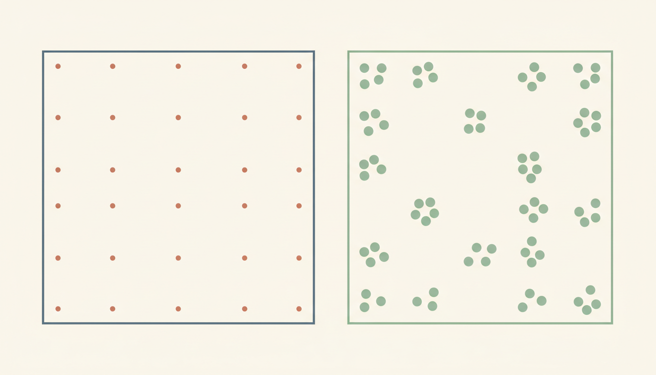
Did you know that a randomly occurring event can have a predictable average count without arriving at predictable times? Imagine an entirely fictional button that flashes an average of two times per hour, independently over disjoint periods with a constant event rate. In the ideal Poisson process model, the chance of no flash in thirty minutes is e⁻¹≈36.79%, while the chance of exactly one flash in the same period is also about 36.79%. Random events can follow precise mathematical distributions.
This Mathematics in Bukit Timah guide explains Poisson counts, rate parameters, independent increments, exponential waiting times, memorylessness, the time to multiple arrivals, superposition, thinning, estimating rates and when a Poisson model fails. Every device, customer, token and observation is fictional. The article does not report Bukit Timah transport arrivals, school activity, queue lengths, local business events, health observations or equipment reliability. We deliberately separate a mathematical point process from actual public schedules or real population behaviour.
Quick answer: For a homogeneous Poisson process with constant rate λ>0 per unit time, the number of events in a time window of length t≥0 is N(t)~Poisson(λt). Thus P(N(t)=k)=e^(−λt)(λt)ᵏ/k!, for nonnegative integers k. The waiting time T to the first event has P(T>t)=e^(−λt) and expected value E[T]=1/λ. These formulas depend on the process’s assumptions; an average observed rate by itself does not prove a real event stream is Poisson.
Article contents
- What is an arrival event?
- Why Bukit Timah is context, not an arrival database
- The rate parameter λ has units
- Worked example 1: change the observation window
- What makes a homogeneous Poisson process?
- Constant rate is not the same as regular spacing
- Worked example 2: distinguish two models
- The Poisson count distribution
- Worked example 3: probability of zero events
- Worked example 4: probability of exactly one event
- Worked example 5: probability of at least two
- Why complements save arithmetic
- Mean and variance are equal for a Poisson count
- Worked example 6: mean and spread for two hours
- Calculate an exact count probability
- Worked example 7: evaluate a Poisson probability
- Poisson probabilities satisfy a recurrence
- Worked example 8: count probabilities when μ equals two
- The probabilities must sum to one
- A time window does not have to begin at zero
- Worked example 9: two equal windows
- Independent increments mean disjoint counts are independent
- Worked example 10: no events across two hours
- Disjoint intervals must be identified correctly
- Worked example 11: overlapping counts
- The waiting time to the first event
- Worked example 12: more than thirty minutes
- The exponential waiting-time cumulative distribution
- Worked example 13: first event within twenty minutes
- Expected waiting time differs from a fixed arrival schedule
- Worked example 14: compare rate and mean wait
- The waiting-time median is shorter than its mean
- Worked example 15: median versus mean
- The memoryless property
- Worked example 16: waiting after one hour
- Why elapsed waiting does not improve the next-step odds here
- Worked example 17: compare two waiting histories
- The exponential density
- Worked example 18: wait between fifteen and thirty minutes
- Variance of an exponential wait
- Worked example 19: waiting spread
- Time to the second event
- Worked example 20: second event within one hour
- The time to the kth event
- Worked example 21: expected third event time
- A Poisson process has no event piles at one exact instant
- Worked example 22: probability of two or more in a short interval
- Two independent Poisson processes can be combined
- Worked example 23: superpose two rates
- Why independence matters in superposition
- Thinning means independently selecting events
- Worked example 24: classify imaginary events
- Conditional event counts lead to binomial structure
- Worked example 25: exactly two Red given three total
- How the Poisson law arises from many rare trials
- Worked example 26: a rare-event approximation
- An average rate alone cannot prove a Poisson model
- Overdispersion is an important diagnostic
- Worked example 27: a deliberately overdispersed toy sequence
- Underdispersion is the opposite pattern
- A time-varying rate requires a different process
- Worked example 28: a linearly increasing fictional rate
- Stationary and independent increments are different properties
- A rate estimated from data has uncertainty
- Worked example 29: use an estimated rate carefully
- Counts in adjacent windows need interpretation
- A Poisson count is not the same as a queue length
- Worked example 30: an invented service distinction
- A scheduled arrival is not Poisson by default
- A comparison of “time until next event” and “time in a queue”
- Poisson events can be counted in other domains
- Time units must be converted before calculations
- Worked example 31: ten minutes at six per hour
- The exponent in e^(−λt) must be dimensionless
- A probability can be checked through limits
- Worked example 32: detect a wrong sign
- The expected count grows linearly with duration
- Worked example 33: double the window
- Interarrival times and event counts are linked
- The model can be simulated without becoming evidence
- Worked example 34: one hypothetical simulated path
- A rare-event approximation has limitations
- A model can fail because events influence future events
- A probability statement should include the full event
- Common error 1: confuse rate with expected count
- Common error 2: treat random arrivals as regular arrivals
- Common error 3: use a count formula for a waiting time
- Common error 4: misunderstand memorylessness
- Common error 5: multiply overlapping window counts
- Common error 6: infer a homogeneous rate from an average alone
- Common error 7: treat expected time as a scheduled time
- Common error 8: ignore time-unit conversion
- Common error 9: confuse interarrival wait with queue-service wait
- Primary preparation: counts and intervals
- Lower Secondary: probability and rates
- Advanced Mathematics and syllabus boundaries
- A twenty-minute family diagnostic
- Seven days of independent practice
- Practice questions with checked answers
- Frequently asked questions
- Official context and connected Mathematics in Bukit Timah

What is an arrival event?
An event is one occurrence in a mathematical counting process.
It could represent a flash in a fictional model or an abstract arrival mark on a timeline. We specify a starting time and then count how many event marks occur over a chosen duration.
The mathematical word “arrival” does not imply a real vehicle timetable or a person’s physical journey. Our events are abstract points on a continuous time axis.
Why Bukit Timah is context, not an arrival database
Families near Beauty World, Sixth Avenue or King Albert Park may be familiar with queues and waiting.
But no actual service intervals or waiting-time observations are provided here. Every rate was invented for arithmetic.
A Poisson process can be useful in applied modelling when its assumptions are defensible, but that is separate from confirming whether any named Singapore service follows the model.
The rate parameter λ has units
If λ=2 events/hour, the number two alone is not sufficient.
The rate specifies expected event counts per hour. Multiplying λ by a duration in hours gives a dimensionless expected count.
For an interval t=0.5 hour, λt=2×0.5=1 expected event. Unit consistency is essential.
Worked example 1: change the observation window
Let λ=2 per hour.
For t=0.5 hour, expected count is 1. For t=2 hours, expected count is 4.
These are mathematical expectations. They do not promise the device will flash exactly one time in the first window or exactly four times in the second.
What makes a homogeneous Poisson process?
In the classic model, events occur at a constant rate λ, and counts in disjoint time intervals are independent.
The distribution of an interval’s count depends only on its length, not where the interval starts. These are independent and stationary increments.
A more formal construction also requires the appropriate small-time behaviour and initial N(0)=0, ensuring a well-defined counting process.
Constant rate is not the same as regular spacing
A clock that flashes exactly once every thirty minutes has a regular deterministic interval.
A Poisson process with rate two per hour has an average of two events per hour, but its gaps are random.
The two processes can have the same long-run average count and very different waiting-time distributions.
Worked example 2: distinguish two models
Model A flashes exactly at minute 30, 60, 90 and so on.
Model B is a homogeneous Poisson process at two events per hour.
Both have rate two per hour in an average sense, but Model A has fixed gaps, whereas Model B has exponential random waiting times. Their formulas are not interchangeable.
The Poisson count distribution
For μ=λt, the number of events in a length-t window has probability
P(N(t)=k)=e^(−μ)μᵏ/k!, where k=0,1,2,…
Here k! is the factorial k×(k−1)×⋯×1, with 0!=1.
The count is discrete even though time is continuous. That distinction matters when choosing a probability formula.
Worked example 3: probability of zero events
Let λ=2/hour and t=0.5 hour, giving μ=1.
For k=0, the formula gives P(N=0)=e⁻¹×1⁰/0!=e⁻¹≈0.367879.
Thus there is about a 36.79% chance of no event in that fictional half-hour under the model.
Worked example 4: probability of exactly one event
Use the same μ=1.
P(N=1)=e⁻¹×1¹/1!=e⁻¹≈0.367879.
Here the zero-event and one-event probabilities happen to be equal because μ=1. That equality does not hold at every rate and duration.
Worked example 5: probability of at least two
For μ=1, probability of two or more events is the complement of zero or one:
P(N≥2)=1−P(N=0)−P(N=1)=1−2e⁻¹.
Numerically that is approximately 0.264241, or 26.42%. All event counts together must account for probability one.
Why complements save arithmetic
The event “at least two” includes k=2,3,4,… without an upper limit.
Summing infinitely many terms directly is unnecessary when the complement contains only zero and one.
Use P(N≥2)=1−P(N=0)−P(N=1). This is a standard probability strategy, not a special property limited to Poisson counts.
Mean and variance are equal for a Poisson count
If X~Poisson(μ), then E[X]=μ and Var(X)=μ.
Its standard deviation is √μ. These are population-model quantities for counts in a fixed duration.
A real count dataset with much larger or much smaller variance than its mean may suggest the simple homogeneous Poisson assumptions are inappropriate.
Worked example 6: mean and spread for two hours
Let λ=3/hour and t=2 hours.
Then μ=6. A Poisson count has expected value 6, variance 6, and standard deviation √6≈2.449.
The count itself can be zero, one, two or any larger nonnegative integer. The model does not guarantee a count near six every time.
Calculate an exact count probability
For μ=6, the probability of exactly four events is
P(N=4)=e⁻⁶6⁴/4!.
Because 6⁴=1,296 and 4!=24, this simplifies to 54e⁻⁶≈0.13385.
The exact symbolic form is useful for verification before numerical rounding.
Worked example 7: evaluate a Poisson probability
Suppose the invented process has rate three per hour and is observed for two hours.
The chance of exactly four events is about 13.39%.
That does not mean the observed count should be 4 or that 13.39% of real physical two-hour periods have been measured to contain four events. It is conditional on the stipulated process.
Poisson probabilities satisfy a recurrence
For X~Poisson(μ) and k≥0,
P(X=k+1)=P(X=k)μ/(k+1).
This follows by dividing consecutive factorial terms.
The recurrence lets a learner build a probability table from P(X=0)=e⁻μ without repeatedly computing large powers and factorials.
Worked example 8: count probabilities when μ equals two
Start P(X=0)=e⁻²≈0.135335.
Then P(X=1)=P(0)×2≈0.270671.
Next P(X=2)=P(1)×2/2≈0.270671. P(X=3)=P(2)×2/3≈0.180447.
The probabilities must sum to one
For a valid Poisson distribution, Σ from k=0 to infinity P(X=k)=1.
The exponential series gives Σ μᵏ/k!=e^μ. Multiplying by e⁻μ returns one.
This is an independent mathematical check on the normalisation of the distribution.
A time window does not have to begin at zero
With stationary increments, an interval from time two to time three has the same Poisson count distribution as an interval from zero to one, provided both last one hour.
The process’s rate is constant in time under the model.
A nonhomogeneous process with changing rate does not have this same stationary-increment property.
Worked example 9: two equal windows
Let λ=2/hour.
The count in the interval [0,1] has Poisson mean two. The count in [4,5] also has Poisson mean two.
That does not make their realised counts equal. It says their probability distributions are the same under the homogeneous model.
Independent increments mean disjoint counts are independent
Let A count events in [0,1] and B count events in [1,2] for a homogeneous Poisson process.
The intervals are disjoint except for a shared endpoint, which has zero probability of an event at that exact preselected instant under the usual model.
Therefore A and B are independent Poisson counts, each with mean λ for one-hour intervals.
Worked example 10: no events across two hours
For λ=2/hour, the probability of no events in the first hour is e⁻².
The probability of no events in the second hour is also e⁻². Independent increments give joint probability e⁻²×e⁻²=e⁻⁴≈0.018316.
The full two-hour count has mean four, so its zero-event probability is likewise e⁻⁴. Both methods agree.
Disjoint intervals must be identified correctly
Overlapping intervals share events and generally have dependent counts.
For example counts in [0,1] and [0,2] are not independent because every event in the first also contributes to the second.
The independent-increments rule applies to nonoverlapping time intervals, not arbitrary windows simply because both have Poisson marginal distributions.
Worked example 11: overlapping counts
Let N(1) count events by hour one, and N(2) count events by hour two.
We always have N(2)≥N(1) because the second total includes the first.
The two random variables therefore cannot be treated as independent ordinary Poisson counts in the way counts from disjoint intervals can.
The waiting time to the first event
Let T be the time from the start of observation until the first arrival.
The event T>t means no arrival occurred during the first t time units.
Thus P(T>t)=P(N(t)=0)=e^(−λt). This directly connects the Poisson count distribution to the exponential waiting-time distribution.
Worked example 12: more than thirty minutes
For λ=2/hour, take t=0.5 hour.
P(T>0.5)=e^(−2×0.5)=e⁻¹≈36.79%.
That is the chance the first arrival is later than thirty minutes, not the chance exactly one arrival occurs in the first thirty minutes.
The exponential waiting-time cumulative distribution
For t≥0, the chance the first event occurs by time t is
P(T≤t)=1−e^(−λt).
This is the complement of surviving beyond t. It is a continuous probability distribution, even though the event counts themselves take integer values.
A particular exact waiting time has probability zero under the continuous model; interval probabilities are the meaningful quantities.
Worked example 13: first event within twenty minutes
Let λ=3/hour. Twenty minutes is 1/3 hour.
Then λt=3×1/3=1. The probability of at least one event by that time is
1−e⁻¹≈0.632121, or about 63.21%.
Expected waiting time differs from a fixed arrival schedule
For T~Exponential(rate λ), E[T]=1/λ.
With λ=2/hour, expected waiting time is 0.5 hour, or thirty minutes.
But the waiting time is not guaranteed to be thirty minutes. It can be shorter or much longer. The mean describes the distribution, not a timetable.
Worked example 14: compare rate and mean wait
At two events per hour, expected first-event wait is 1/2 hour.
At four events per hour, expected wait is 1/4 hour.
Doubling the rate halves the mean exponential waiting time under this model. That does not establish actual waits for any real public service.
The waiting-time median is shorter than its mean
For an exponential waiting time, the median m satisfies P(T≤m)=0.5.
Thus 1−e^(−λm)=0.5, giving m=ln2/λ.
Because ln2≈0.693<1, the median is less than the mean 1/λ. The exponential distribution is right-skewed.
Worked example 15: median versus mean
Let λ=2/hour.
Mean waiting time is 1/2 hour=30 minutes.
Median is ln2/2 hour≈0.34657 hour≈20.79 minutes. Half of the model waiting times end before that median, even though the average wait is longer.
The memoryless property
The exponential distribution satisfies
P(T>s+t | T>s)=P(T>t) for s,t≥0.
In words, conditional on having waited longer than s without an event, the distribution of the additional wait is unchanged.
This is a special mathematical property of the exponential waiting model; it is not a universal statement about all real queues or scheduled arrivals.
Worked example 16: waiting after one hour
For λ=2/hour, suppose no event has occurred during the first hour.
The chance of waiting another 0.5 hour with no event is
e^(−2×0.5)=e⁻¹≈36.79%.
It is the same as the probability of no arrival in a fresh half-hour interval under the homogeneous Poisson model.
Why elapsed waiting does not improve the next-step odds here
For a regular timetable, knowing how long you have waited may help predict the next scheduled event.
For a homogeneous Poisson process, the memoryless distribution says the extra waiting time has the same law after any completed waiting period.
These processes behave differently. One should not transfer the memoryless rule to actual services without evidence.
Worked example 17: compare two waiting histories
Imagine two tokens. Token A starts waiting now. Token B has already waited forty minutes without an event.
Under the same rate-two Poisson model, their probability of seeing an event in the next fifteen minutes is 1−e^(−2×0.25)=1−e⁻⁰·⁵≈39.35%.
The prior elapsed time does not change that conditional next-window probability in this model.
The exponential density
For t≥0, the exponential waiting-time density is
f_T(t)=λe^(−λt).
Its value has units reciprocal time, and it should not be mistaken for the probability of an exact instant.
Integrating the density over an interval [a,b] gives the probability that the waiting time lies between those two times.
Worked example 18: wait between fifteen and thirty minutes
Let λ=2/hour, a=0.25 hour and b=0.5 hour.
P(a<T≤b)=P(T>a)−P(T>b)=e^(−0.5)−e^(−1).
Numerically that is approximately 0.606531−0.367879=0.238652, or 23.87%.
Variance of an exponential wait
For T~Exponential(rate λ),
Var(T)=1/λ² and standard deviation is 1/λ.
Thus its standard deviation equals its mean under this model.
This differs from a Poisson count, where variance equals the mean numerically. Their units are also different: count variance versus squared time variance.
Worked example 19: waiting spread
For λ=2/hour, E[T]=0.5 hour.
Variance is 1/4 hour², and standard deviation is 0.5 hour.
The relatively large standard deviation reflects the broad, right-skewed waiting distribution. It does not mean every wait stays within half an hour of the mean.
Time to the second event
Let S₂ be the waiting time from the starting point until two events have occurred.
It is the sum of two independent exponential interarrival times under the Poisson model.
Its distribution is Gamma with shape two and rate λ, also called Erlang-2. Its expected value is 2/λ.
Worked example 20: second event within one hour
With λ=2/hour, the second event has occurred by one hour exactly when N(1)≥2.
That probability is
1−P(N(1)=0)−P(N(1)=1)=1−e⁻²−2e⁻²=1−3e⁻².
Numerically it is approximately 0.593994, or 59.40%.
The time to the kth event
For a homogeneous Poisson process, the waiting time Sₖ until the kth event has a Gamma distribution with integer shape k and rate λ.
Its mean is E[Sₖ]=k/λ, and its variance is k/λ².
The count and waiting-time formulations are connected by P(Sₖ≤t)=P(N(t)≥k).
Worked example 21: expected third event time
Let λ=2/hour.
The expected time until the third event is 3/2 hours, or ninety minutes.
This is not a guaranteed third event at precisely ninety minutes. It is the mean of a random waiting-time distribution.
A Poisson process has no event piles at one exact instant
In the ordinary simple homogeneous Poisson process, the probability of two or more events occurring within a very short interval decreases on the order of the interval length squared.
This is part of why the model treats arrivals as isolated random points in continuous time.
Real systems can generate simultaneous batches, so such systems may require compound or clustered process models.
Worked example 22: probability of two or more in a short interval
Let μ=λh for a short interval h.
P(N≥2)=1−e⁻μ(1+μ).
For small μ, this is approximately μ²/2 to leading order. The quadratic leading behaviour makes multiple arrivals much rarer than one arrival over sufficiently short intervals.
Two independent Poisson processes can be combined
Suppose invented event stream A is homogeneous Poisson at λ₁ and independent event stream B is homogeneous Poisson at λ₂.
Their combined events form a Poisson process at rate λ₁+λ₂, under the standard superposition assumptions.
This gives a clean way to combine independent sources without computing every possible count split directly.
Worked example 23: superpose two rates
Let stream A have rate two per hour and stream B rate three per hour.
The combined rate is five events per hour.
In a one-hour interval, the total count is Poisson with mean five. Its zero-event probability is e⁻⁵≈0.006738.
Why independence matters in superposition
If two devices always flash simultaneously, their total counts are correlated and may occur in batches.
Adding their marginal rates is still a calculation of expected combined count if counted appropriately, but the resulting process need not be an ordinary simple Poisson process.
The theorem requires independent underlying Poisson processes, not merely two rates written on a page.
Thinning means independently selecting events
Suppose each event in a rate-λ Poisson process is independently labelled Red with probability p and Blue with probability 1−p.
The Red events form a Poisson process with rate pλ, and the Blue events form an independent Poisson process with rate (1−p)λ, under the standard thinning theorem.
This is a conditional mathematical result requiring independent labels.
Worked example 24: classify imaginary events
Let the original rate be six per hour.
Independently label each event Red with probability one-third. The Red rate is 2 per hour; the other rate is 4 per hour.
A thirty-minute interval has expected Red count one and expected other count two. The labels are abstract categories, not real traffic types.
Conditional event counts lead to binomial structure
If N(t)=n total Poisson events occurred, and each is independently labelled Red with probability p, the Red count conditional on n is Binomial(n,p).
Unconditionally, the Red count is Poisson with mean pλt.
This connection explains how binomial classification and Poisson counts combine, under independent marking.
Worked example 25: exactly two Red given three total
Suppose three fictional events occurred and each is independently labelled Red with probability one-half.
Conditional probability of exactly two Red labels is C(3,2)(1/2)²(1/2)=3/8.
This is binomial because the total number of trials is now fixed at three. The unconditional event total remains Poisson.
How the Poisson law arises from many rare trials
Consider n independent Bernoulli trials, each with small success probability p=μ/n.
The count is Binomial(n,μ/n).
As n→∞ with μ fixed, that binomial distribution approaches Poisson(μ). This rare-event limit provides one mathematical motivation for Poisson counts.
Worked example 26: a rare-event approximation
Suppose a toy experiment has 1,000 independent opportunities, each with probability 0.002 of a counted event.
Its binomial expected count is 1,000×0.002=2.
Poisson(2) may approximate the count distribution, including P(X=0)≈e⁻². Whether the approximation is adequate depends on the model and required accuracy.
An average rate alone cannot prove a Poisson model
A machine that flashes exactly every thirty minutes has rate two per hour.
A Poisson process with rate two per hour also has that expected rate, but its timing and count variability are different.
An observed mean cannot establish independent increments, stationarity or exponential interarrival times. Those assumptions need their own evidence.
Overdispersion is an important diagnostic
In a Poisson count model, mean equals variance.
If counts in equal-length windows have variance consistently much greater than their mean, this may indicate clustering, changing rates or heterogeneous conditions.
One should consider alternative models or investigate data quality rather than simply force a Poisson distribution because event counts are nonnegative integers.
Worked example 27: a deliberately overdispersed toy sequence
Imagine four fictional equal-window counts: 0,0,0,12.
Their sample mean is three. Their population-style average squared deviation is (9+9+9+81)/4=27, far larger than three.
This toy distribution is not characteristic of a well-fitting constant-rate Poisson count model, although four observations alone cannot establish a definitive population distribution.
Underdispersion is the opposite pattern
If event counts vary much less than their mean, a rigid timing mechanism or capacity constraint may be present.
Regularly scheduled events are less random than the independent-increment Poisson model in relevant ways.
The variance-to-mean comparison is a diagnostic clue, not a complete statistical goodness-of-fit proof.
A time-varying rate requires a different process
Some event intensities change with time.
A nonhomogeneous Poisson process with deterministic rate λ(t)≥0 uses independent increments but generally does not have stationary increments.
The mean number of events over [a,b] is ∫ from a to b λ(u)du, not necessarily a constant λ times interval length.
Worked example 28: a linearly increasing fictional rate
Suppose λ(t)=2+t events/hour for t measured in hours over [0,2].
The mean count from zero to two is
∫₀²(2+t)dt=[2t+t²/2]₀²=4+2=6.
Under the nonhomogeneous Poisson model, the count in that interval is Poisson with mean six. The rate is not constant, so equal-length windows at different times need not have the same distribution.
Stationary and independent increments are different properties
Stationary increments mean the count distribution depends only on interval length.
Independent increments mean counts over disjoint intervals are independent.
A homogeneous Poisson process has both. A nonhomogeneous Poisson process still has independent increments, but its distributions vary with the time-dependent integrated rate.
A rate estimated from data has uncertainty
Suppose a fictional observer records 18 events over six hours.
The crude estimated average rate is 18/6=3 per hour.
That estimate is not proof the true underlying constant rate equals three, nor proof the events form a Poisson process. Statistical inference would require an appropriate observation and sampling model.
Worked example 29: use an estimated rate carefully
If a homogeneous rate-three-per-hour Poisson model is provisionally assumed, the expected count in twenty minutes is one.
Then the model predicts P(no events in twenty minutes)=e⁻¹.
A report should say “under the fitted model” and acknowledge that rate estimation and model fit are uncertain, rather than claiming the next event time is known.
Counts in adjacent windows need interpretation
For a genuine homogeneous Poisson process, disjoint equal-duration windows have independent identically distributed Poisson counts.
If observations display strong serial dependence, repeating cycles or changing average intensity, the homogeneous model may be inappropriate.
Do not use independent-increment formulas simply because the dataset is organised in equal-sized rows.
A Poisson count is not the same as a queue length
N(t) counts the number of arrivals in a specified time interval.
A queue length depends on both arrivals and departures or service completions, as well as initial conditions and capacity.
Two systems can have identical arrival processes but very different queues when service rates differ. Arrival count alone does not determine waiting in an actual service system.
Worked example 30: an invented service distinction
Suppose two fictional counters each receive events at the same Poisson arrival rate.
One processes items almost instantly; the other processes items slowly. Even with identical arrival rates, their queue lengths and time in system can differ substantially.
This is why our exponential interarrival waiting must not be called the waiting time for service without an additional queueing model.
A scheduled arrival is not Poisson by default
Actual buses and trains may follow published or operationally controlled schedules, even if delays introduce uncertainty.
Their arrival processes are not automatically memoryless and their waits may depend on service headways, time of day and current information.
The mathematics in this guide cannot provide real-time transport availability or expected walking routes.
A comparison of “time until next event” and “time in a queue”
The first-event waiting time in a rate-λ Poisson process is exponential with mean 1/λ.
Time spent awaiting service in a queue additionally depends on service discipline, processing times and how many customers are already waiting.
They are different random variables. Giving them the same name would be a model error.
Poisson events can be counted in other domains
The mathematical process can model abstract event times, random failures under suitable reliability assumptions or simulated arrivals.
Each application needs a justified rate, independence structure and observation window.
One should not assume a real system has independent events merely because its data are expressed as small integer counts.
Time units must be converted before calculations
If λ is stated per hour, a duration t of ten minutes is 1/6 hour.
Using t=10 directly without converting would model ten hours rather than ten minutes.
The mean count λt must be dimensionless. Unit checking is a first-line diagnostic for mistakes in these formulas.
Worked example 31: ten minutes at six per hour
Let λ=6 per hour and t=10/60=1/6 hour.
Then μ=6×1/6=1.
The probability of zero events is e⁻¹ and of at least one is 1−e⁻¹. Using t=10 without unit conversion would yield μ=60 and a completely different answer.
The exponent in e^(−λt) must be dimensionless
The rate λ has units inverse time, while t has units time.
Their product λt has no units, making it a valid exponential argument.
If a calculation produces an exponent of “six events per hour” without multiplying by a compatible duration, the probability expression is dimensionally incomplete.
A probability can be checked through limits
For a homogeneous Poisson process with λ>0, P(N(t)=0)=e^(−λt).
At t=0, this equals one: no time has passed, so no event occurred.
As t becomes very large, the probability approaches zero. These limiting checks agree with the model and help catch a misplaced sign in the exponent.
Worked example 32: detect a wrong sign
A pupil writes P(no events)=e^(+λt).
For any t>0, λ>0, this exceeds one, which is impossible for a probability.
The correct formula is e^(−λt). Its values lie between zero and one, decreasing as the observation window grows.
The expected count grows linearly with duration
Under constant λ, E[N(t)]=λt.
Doubling t doubles the expected count. But it does not double every individual realised count.
The count’s variance also grows linearly with t, while standard deviation grows like √t. These different scaling laws reveal more about the distribution.
Worked example 33: double the window
At λ=2/hour, a one-hour count has mean two and SD √2.
A two-hour count has mean four and SD two.
The mean doubles, but the SD increases by factor √2, not by two. The underlying distribution changes with the window size.
Interarrival times and event counts are linked
If W₁,W₂,… are independent exponential waits with rate λ, event n occurs at Sₙ=W₁+⋯+Wₙ.
The count N(t) is the largest n such that Sₙ≤t, with the usual zero count if no event has occurred.
This connection describes one Poisson process through two perspectives: counting events by time or waiting for successive events.
The model can be simulated without becoming evidence
A computer can sample exponential waits and accumulate them until a chosen observation horizon.
The resulting simulated event times will vary from run to run.
Simulation is useful for testing understanding, but synthetic data do not validate the model against any real Bukit Timah device, service or population.
Worked example 34: one hypothetical simulated path
Suppose a fictional sample of waiting times is 0.1,0.4,0.2,0.7 hours.
The cumulative event times are 0.1,0.5,0.7,1.4 hours.
There are three events by t=1 hour and four by t=1.5 hours. This is one constructed path, not a probability prediction or observation.
A rare-event approximation has limitations
The binomial-to-Poisson approximation assumes many independent opportunities with small individual event chances and a stable total mean.
Strong dependence, clustered failures or changing opportunity probabilities can undermine that approximation.
Do not infer a Poisson process merely because a single count histogram looks roughly right. Time structure matters too.
A model can fail because events influence future events
In a self-exciting process, one occurrence may make later occurrences more likely in the near term.
Then the future rate depends on recent history, violating the simple independent-increments assumption.
Other process models exist for such effects. Our constant-rate Poisson formulas are deliberately limited to the simpler case.
A probability statement should include the full event
“Probability 0.37” is incomplete without identifying the interval, rate and event type.
For our half-hour rate-two example, 0.3679 represents both exactly zero and exactly one event by numerical coincidence.
A good mathematical report states P(N(0.5)=0) or P(N(0.5)=1) rather than treating the numerical value as self-explanatory.
Common error 1: confuse rate with expected count
A rate of two per hour does not imply two events in every half-hour.
The expected count for thirty minutes is one, found by multiplying rate by 0.5 hour.
State λ and t separately before computing μ=λt.
Common error 2: treat random arrivals as regular arrivals
A homogeneous Poisson process has exponentially distributed interarrival times.
It is not a deterministic event every 1/λ time units.
The average rate and the spacing distribution are different aspects of the model.
Common error 3: use a count formula for a waiting time
N(t) takes integer values and has a Poisson distribution.
The first waiting time T is continuous and has an exponential distribution.
Selecting the wrong distribution can produce nonsensical probabilities such as asking P(T=3) with a Poisson count formula.
Common error 4: misunderstand memorylessness
Exponential memorylessness concerns the additional waiting time conditional on surviving so far.
It does not claim the probability of surviving a longer total interval is unchanged.
For example P(T>1.5) is smaller than P(T>0.5), though P(T>1.5|T>1)=P(T>0.5).
Common error 5: multiply overlapping window counts
Independent increments apply to disjoint intervals.
N(1) and N(2) share the first hour’s events, so they are not independent in the usual nondegenerate Poisson model.
Distinguish cumulative totals from increments over separate intervals.
Common error 6: infer a homogeneous rate from an average alone
An observed rate of three per hour may come from a periodic device, a clustered process or changing-rate activity.
A Poisson model requires more structure than one average statistic.
Use data and model checks rather than presenting the count formula as universally appropriate.
Common error 7: treat expected time as a scheduled time
At λ=2 per hour, mean wait is thirty minutes, but the process has a broad distribution.
No individual next event is guaranteed at thirty minutes.
The result is not a timetable and should not be used as a real transport arrival estimate.
Common error 8: ignore time-unit conversion
A duration of fifteen minutes is one-quarter of an hour.
For λ=4/hour, the expected count in that interval is one, not sixty.
Incorrect units can change the Poisson exponent and every subsequent probability.
Common error 9: confuse interarrival wait with queue-service wait
The exponential first-event wait is time until the next counted event.
A person’s service wait in a queue depends on backlog and service dynamics as well.
One cannot infer actual queue delay from an arrival rate alone.
Primary preparation: counts and intervals
Younger pupils can record how many invented marks occur in different time boxes and notice that equal-length windows need not have the same count.
They can distinguish average counts from a guaranteed count.
Formal exponential distributions should follow after confidence with fractions, graphs and simple probability.
Lower Secondary: probability and rates
Students can calculate rate×time, use complements and distinguish discrete counts from continuous durations.
They can compare regular and random timing models conceptually without memorising Gamma distributions.
Algebraic work with eˣ, factorials and continuous probability belongs to later learning pathways.
Advanced Mathematics and syllabus boundaries
Poisson processes and exponential waiting times are advanced probability and stochastic-process enrichment.
The SEAB 2027 G3 Mathematics and Additional Mathematics syllabus directory provides Secondary foundations; the 2027 A-Level syllabus directory provides further pathways.
The full point-process model is not claimed to be mandatory for every SEC G3 learner.
A twenty-minute family diagnostic
Minutes 1–5: Convert thirty minutes to half an hour and calculate μ=2×0.5=1.
Minutes 6–10: Find P(N=0)=e⁻¹, P(N=1)=e⁻¹ and P(N≥2)=1−2e⁻¹.
Minutes 11–15: Derive P(T>t)=P(N(t)=0)=e^(−λt). Find expected wait 1/λ.
Minutes 16–20: Compare a regular flash every thirty minutes with a Poisson rate-two process. Explain why the same average does not prove the same waiting model.
Seven days of independent practice
Day one revises rates and time conversion. Day two computes Poisson probabilities.
Day three uses complements and Poisson recurrence. Day four derives exponential waiting probabilities. Day five studies memorylessness.
Day six combines and thins independent Poisson streams. Day seven diagnoses an invented clustered or scheduled process that violates homogeneous Poisson assumptions.
Practice questions with checked answers
A. λ=2/hour and t=0.5 hour: expected count? Answer: 1.
B. Same window, P(N=0)? Answer: e⁻¹≈0.367879.
C. Same window, P(N≥2)? Answer: 1−2e⁻¹≈0.264241.
D. λ=3/hour over two hours: mean count? Answer: 6.
E. For Poisson mean six, P(N=4)? Answer: 54e⁻⁶≈0.13385.
F. λ=2/hour, mean first waiting time? Answer: 0.5 hour.
G. λ=2/hour, first-wait median? Answer: ln2/2 hour≈20.79 minutes.
H. λ=2/hour, second event by one hour? Answer: 1−3e⁻²≈0.593994.
Frequently asked questions
What is a Poisson process?
A continuous-time counting model with appropriate independent increments and a constant rate in its homogeneous form.
Does rate two mean exactly two events every hour?
No. It means the expected count is two per hour; realised counts follow a probability distribution under the model.
Which distribution describes the number of events?
The count over a fixed interval is Poisson with mean λt.
Which distribution describes the waiting time to the first event?
It is exponential with rate λ, under a homogeneous Poisson process.
What does memoryless mean?
After waiting without an event, the distribution of additional waiting time is unchanged in the exponential model.
What is the expected first-event wait?
1/λ in the matching time units.
Do separate time windows have independent counts?
Yes for disjoint intervals under the homogeneous Poisson model. Overlapping cumulative windows do not have that independence.
Can two independent Poisson streams be combined?
Yes. Their superposition is Poisson with the sum of their rates under the stated independent-process assumptions.
Are these actual Bukit Timah public-transport or school statistics?
No. All rates, flash events, observation windows and numerical outcomes are fictional.
How can parents recognise understanding?
The learner can convert time units, separate counts from waiting times, use complements correctly and explain why a constant average rate does not establish a Poisson process.
Official context and connected Mathematics in Bukit Timah
Use the SEAB 2027 G3 Mathematics and Additional Mathematics syllabus directory for the actual school-level scope. The complete Poisson process model here is enrichment with invented rates and observations, not a real service or statistical report.
Continue with Queue Length, Service Rates and Waiting Time, Probability, Independence and Fair Games, Expected Values and Probability Distributions, Exponential Models and Doubling Time and Markov Chains and Transition Probabilities for related but distinct ideas.
The immutable Clementi Secondary 1 Mathematics small-group teaching reference anchors first-principles explanations, checked worked examples, diagnosis of errors and independent transfer.
The lasting habit is to define the counted event and rate units, distinguish random counts from waiting times, verify the independent-increment assumptions and never convert a hypothetical event model into an unverified local schedule.
Companion Mathematics in Bukit Timah lessons in this four-article batch: Pigeonhole Principle, Guaranteed Matches and Counting Proofs · Generating Functions, Coefficients and Recursive Counting · Jensen’s Inequality, Convexity and Why Averages Behave Differently. These new guides connect deterministic counting, generating functions, convex averages and stochastic processes, each with original fictional worked examples and carefully stated assumptions.