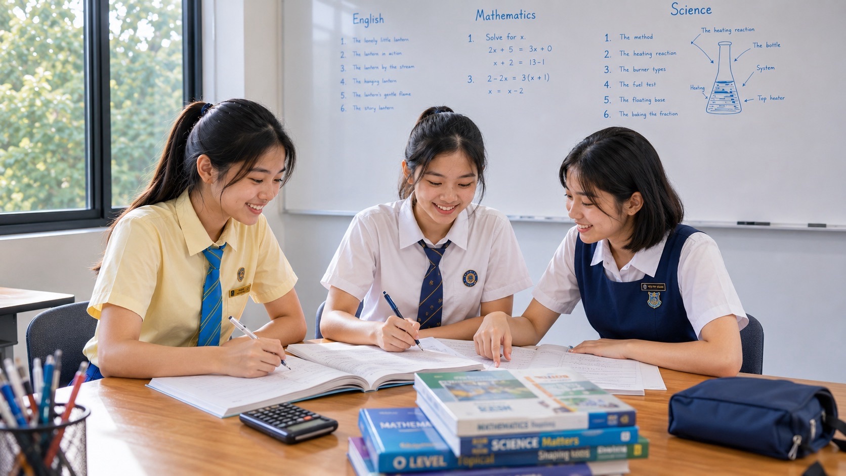
WHY MATHEMATICS?

Why Mathematics? | NicheCompass Cell Niches: Variational Graph Autoencoders, Latent Programs, Masked Decoders and KL Divergence

How NicheCompass combines spatial neighbours, molecular measurements and prior gene programs to learn interpretable probabilistic niche representations that can transfer across samples.

Why mathematics is important becomes easier to see when a real decision depends on it. This guide follows the mechanism from definitions and dimensions to a worked calculation, validation, practical learning and responsible use. It keeps factual evidence separate from interpretation and treats every illustrative scenario as an example rather than a promise of results.

Choose a reading route

Encode self and neighbourhood molecular context
Use mean, variance and reparameterized latent samples
Reconstruct graphs and omics through masked decoders
Balance reconstruction, KL regularization and program sparsity

Chapter map

1. Spatial adjacency matrix
2. Self-omics matrix
3. Neighbour-omics aggregate
4. Prior gene-program mask
5. Graph encoder
6. Latent mean and log-variance
7. Standard Normal prior
8. Reparameterization trick
9. Graph decoder
10. Self-omics masked decoder
11. Neighbour-omics masked decoder
12. Reconstruction loss
13. KL divergence
14. De novo program
15. Selective pruning
16. Niche embedding and transfer

Visit the How Mathematics Works hub for the wider series and its connections to education, reasoning, science, computing, design and careers.

1. Spatial adjacency matrix

Here the geometry becomes operational. A binary or weighted matrix records declared neighbours.

A concrete situation

Aij equals one for adjacent cells.

What the mathematics does not license

Neighbour rules change the niche. The habit of checking assumptions is one of the practical benefits of learning mathematics.

Try it, check it, transfer it

Sweep radii and graph types. Then explain the result to someone who has not seen the formula. If the explanation needs a hidden assumption, add that assumption to the model record.

2. Self-omics matrix

This step deserves a careful pause. Each cell contributes its own measured feature vector.

A concrete situation

Cell i has expression x-i.

What the mathematics does not license

Counts carry technical noise. The same reasoning helps students move from an exercise to a real dataset.

Try it, check it, transfer it

Model offsets and transformations. Then explain the result to someone who has not seen the formula. If the explanation needs a hidden assumption, add that assumption to the model record.

3. Neighbour-omics aggregate

The useful question is not only how to calculate, but what the calculation assumes. Graph neighbours contribute an aggregated context vector.

A concrete situation

Mean neighbour expression is x-prime-i.

What the mathematics does not license

A mean hides heterogeneous senders. That distinction matters because a correct formula can still answer the wrong operational question.

Try it, check it, transfer it

Inspect distributions and weights. Then explain the result to someone who has not seen the formula. If the explanation needs a hidden assumption, add that assumption to the model record.

4. Prior gene-program mask

A small example makes the mechanism visible. A binary mask links programs to documented genes.

A concrete situation

Program p connects to 40 genes.

What the mathematics does not license

Knowledge bases are incomplete. The habit of checking assumptions is one of the practical benefits of learning mathematics.

Try it, check it, transfer it

Version and audit masks. Then explain the result to someone who has not seen the formula. If the explanation needs a hidden assumption, add that assumption to the model record.

Did You Know? In this chapter, the most important number is useful only together with its construction rule. Changing scaling, sample membership or validation design can change the numerical answer without changing the arithmetic.

5. Graph encoder

This is where modelling choices begin to affect evidence. Message passing combines self and neighbour evidence.

A concrete situation

Two layers produce hidden vector h-i.

What the mathematics does not license

Oversmoothing can merge niches. The same reasoning helps students move from an exercise to a real dataset.

Try it, check it, transfer it

Compare layer depth. Then explain the result to someone who has not seen the formula. If the explanation needs a hidden assumption, add that assumption to the model record.

6. Latent mean and log-variance

The central mathematical idea is concrete. The encoder outputs distribution parameters.

A concrete situation

mu equals 0.5 and log variance -0.7.

What the mathematics does not license

Variance can collapse. That distinction matters because a correct formula can still answer the wrong operational question.

Try it, check it, transfer it

Plot per-program uncertainty. Then explain the result to someone who has not seen the formula. If the explanation needs a hidden assumption, add that assumption to the model record.

7. Standard Normal prior

Here the geometry becomes operational. Latent variables are regularized toward N(0,I).

A concrete situation

Prior mean zero and variance one.

What the mathematics does not license

The prior may be too simple. The habit of checking assumptions is one of the practical benefits of learning mathematics.

Try it, check it, transfer it

Check posterior mismatch. Then explain the result to someone who has not seen the formula. If the explanation needs a hidden assumption, add that assumption to the model record.

8. Reparameterization trick

This step deserves a careful pause. A sample is mu plus sigma times random epsilon.

A concrete situation

0.5 plus 0.7 times epsilon.

What the mathematics does not license

Randomness adds training variance. The same reasoning helps students move from an exercise to a real dataset.

Try it, check it, transfer it

Use repeated seeds. Then explain the result to someone who has not seen the formula. If the explanation needs a hidden assumption, add that assumption to the model record.

9. Graph decoder

The useful question is not only how to calculate, but what the calculation assumes. Latent vectors predict spatial adjacency.

A concrete situation

A sigmoid of z-i dot z-j predicts an edge.

What the mathematics does not license

Nearby cells need not share state. That distinction matters because a correct formula can still answer the wrong operational question.

Try it, check it, transfer it

Evaluate edge calibration. Then explain the result to someone who has not seen the formula. If the explanation needs a hidden assumption, add that assumption to the model record.

10. Self-omics masked decoder

A small example makes the mechanism visible. Program activities reconstruct each cell’s own features.

A concrete situation

z times masked weights predicts x.

What the mathematics does not license

Mask errors bias interpretation. The habit of checking assumptions is one of the practical benefits of learning mathematics.

Try it, check it, transfer it

Compare with relaxed masks. Then explain the result to someone who has not seen the formula. If the explanation needs a hidden assumption, add that assumption to the model record.

11. Neighbour-omics masked decoder

This is where modelling choices begin to affect evidence. Latent programs reconstruct neighbourhood context.

A concrete situation

z predicts x-prime through a second mask.

What the mathematics does not license

Self and neighbour signals are dependent. The same reasoning helps students move from an exercise to a real dataset.

Try it, check it, transfer it

Report each loss separately. Then explain the result to someone who has not seen the formula. If the explanation needs a hidden assumption, add that assumption to the model record.

12. Reconstruction loss

The central mathematical idea is concrete. Graph and omics errors reward data fit.

A concrete situation

Binary cross-entropy plus count loss.

What the mathematics does not license

Large modalities can dominate. That distinction matters because a correct formula can still answer the wrong operational question.

Try it, check it, transfer it

Publish loss weights. Then explain the result to someone who has not seen the formula. If the explanation needs a hidden assumption, add that assumption to the model record.

13. KL divergence

Here the geometry becomes operational. The posterior is penalized for departing from the prior.

A concrete situation

KL for one diagonal Gaussian is calculated analytically.

What the mathematics does not license

High KL weight can erase signal. The habit of checking assumptions is one of the practical benefits of learning mathematics.

Try it, check it, transfer it

Plot a beta sweep. Then explain the result to someone who has not seen the formula. If the explanation needs a hidden assumption, add that assumption to the model record.

14. De novo program

This step deserves a careful pause. Unmasked latent factors capture missing prior biology.

A concrete situation

Program d loads on an unseen gene set.

What the mathematics does not license

Flexible factors can absorb artefacts. The same reasoning helps students move from an exercise to a real dataset.

Try it, check it, transfer it

Require stability and annotation. Then explain the result to someone who has not seen the formula. If the explanation needs a hidden assumption, add that assumption to the model record.

15. Selective pruning

The useful question is not only how to calculate, but what the calculation assumes. Weak program-gene weights are regularized and removed.

A concrete situation

Weights below a rule are pruned.

What the mathematics does not license

Pruning thresholds change meaning. That distinction matters because a correct formula can still answer the wrong operational question.

Try it, check it, transfer it

Record the full path. Then explain the result to someone who has not seen the formula. If the explanation needs a hidden assumption, add that assumption to the model record.

16. Niche embedding and transfer

A small example makes the mechanism visible. Latent activities align cells across samples.

A concrete situation

A query cell maps near reference niche two.

What the mathematics does not license

Batch alignment can erase novelty. The habit of checking assumptions is one of the practical benefits of learning mathematics.

Try it, check it, transfer it

Hold out tissues and inspect unmatched cells. Then explain the result to someone who has not seen the formula. If the explanation needs a hidden assumption, add that assumption to the model record.

A seven-day practice lab

Day 1: define the decision, observation unit, X variables and Y or reference condition.
Day 2: reproduce the smallest worked example and check every dimension, unit and sign.
Day 3: build a transparent baseline and write what it assumes.
Day 4: fit the main method inside a training-only pipeline; record every parameter.
Day 5: challenge one assumption with a deliberately difficult dataset or operating regime.
Day 6: compare validation metrics with the practical workload created by errors.
Day 7: present one supported conclusion, one unresolved uncertainty and one safe next experiment.

Questions for a student, parent or mentor

Which part of the model is a mathematical definition, and which part is a choice?
What small calculation would catch a sign, scale or dimension error?
What evidence comes from training, validation and the untouched test?
What benign condition could look like a fault or prediction failure?
How would the answer change for another response, asset, school project or time period?
What should a human review before acting on the score?

A method-specific audit before deployment

NicheCompass learns a spatial niche representation with a conditional variational graph autoencoder. The encoder sees molecular features together with a spatial neighbour graph and produces a mean and log-variance for every cell in a latent space. Sampling through the reparameterization trick lets gradients train the model while retaining a probability distribution for each cell’s latent state.

The latent variables have a standard Normal prior. A Kullback-Leibler divergence term discourages the approximate posterior from drifting arbitrarily far from that prior, while reconstruction terms reward accurate recovery of observed structure. The balance between those terms controls whether the model memorizes details or produces an overly smooth latent map. A tidy embedding is not automatically a faithful one.

Interpretability comes from masked decoders linked to prior gene programs. Separate decoders reconstruct a cell’s own molecular state and neighbourhood-aggregated state. Binary masks restrict many decoder weights to known program-gene relationships, while de novo programs can capture patterns missing from the prior knowledge. Selective regularization and pruning keep those extra programs from becoming an unrestricted explanation for everything.

A graph decoder also reconstructs spatial adjacency from the latent representation. This joins molecular and neighbourhood evidence in one training objective, making the learned coordinates useful for niche discovery and reference mapping. Validation must still separate donors or tissues, compare alternative neighbourhood graphs, inspect program stability and report uncertainty. Latent proximity describes modelled similarity, not direct contact or common fate.

Frequently asked questions

What is NicheCompass?

NicheCompass is a conditional variational graph-autoencoder framework for interpretable spatial niche representation and integration.

What is a latent gene program?

It is a latent dimension connected to a set of genes through prior masks or learned de novo relationships.

Why is the encoder variational?

It learns a distribution described by a mean and variance for each cell rather than one fixed coordinate.

What does KL divergence do?

It regularizes the approximate latent posterior toward a standard Normal prior, limiting unrestricted memorization.

Why use masked decoders?

Masks restrict many weights to biologically defined program-gene connections, making latent activities easier to interpret.

Does a niche embedding prove a biological niche?

No. It is a model-derived representation that needs spatial, molecular and cross-sample validation.

Primary source and fact-check note

Sebastian Birk, Irene Bonafonte-Pardàs, Adib Miraki Feriz, Adam Boxall, Eneritz Agirre, Fani Memi, Anna Maguza, Anamika Yadav, Erick Armingol, Rong Fan, Gonçalo Castelo-Branco, Fabian J. Theis, Omer Ali Bayraktar, Carlos Talavera-López, Mohammad Lotfollahi et al., “Quantitative characterization of cell niches in spatially resolved omics data,” Nature Genetics 57, 897–909 (2025), DOI 10.1038/s41588-025-02120-6. Definitions and core claims in this article were checked against this primary publication. Calculations shown here were independently recomputed. Examples are educational illustrations; they are not reported industrial performance results.

Useful next reading

Keep the options open. Mathematics education supports clearer questions, transferable problem-solving skills and informed choices across science, engineering, computing, AI, statistics, design and many other careers. It does not guarantee intelligence, income, admission or employment; those outcomes depend on far more than one subject or model.

Extended laboratory: topic-specific validation and responsible use

Adjacency audit

Version neighbour graph construction and density.

Encoder audit

Publish layers, hidden sizes and oversmoothing checks.

Posterior audit

Inspect means, variances and latent collapse.

Mask audit

Version prior programs and relaxed-mask comparisons.

Did You Know? A sophisticated adjustment can be algebraically correct and still answer the wrong scientific question when samples, labels, batches or validation boundaries are wrong.

Loss audit

Separate graph, self-omics, neighbour-omics and KL terms.

De novo audit

Require stability for unmasked programs.

Transfer audit

Test unmatched query cells and held-out tissues.

Final claim

A latent niche is a model representation, not observed identity.

Did You Know? A sophisticated adjustment can be algebraically correct and still answer the wrong scientific question when samples, labels, batches or validation boundaries are wrong.

Mechanism workshop: calculate, challenge and transfer

Workshop 1: Spatial adjacency matrix

Begin with this mechanism: A binary or weighted matrix records declared neighbours. Recreate the concrete case: Aij equals one for adjacent cells. Write adjacency entries, self features, neighbour aggregates, mask values, latent means, variances, samples, reconstructions, KL terms and program activities with direction, units, denominators and assumptions. Calculate the smallest non-trivial example by hand, then reproduce it in a spreadsheet or short program. Challenge this limitation: Neighbour rules change the niche. Complete the transfer step: Sweep radii and graph types. Change exactly one catalogue, normalization, threshold, neighbourhood radius, distance kernel, graph layer, hidden dimension, attention seed, corruption rule, latent prior, decoder mask, KL weight, sender bag, spatial metric, shrinkage prior or validation split. Explain which mathematical object changes, which conclusion survives and which claim must weaken. Keep measurement, graph construction, probabilistic assumption, optimization, prediction, interpretation and validation on separate notebook lines. Reserve whole donors, tissues or conditions outside tuning when testing transfer.

Workshop 2: Self-omics matrix

Begin with this mechanism: Each cell contributes its own measured feature vector. Recreate the concrete case: Cell i has expression x-i. Write adjacency entries, self features, neighbour aggregates, mask values, latent means, variances, samples, reconstructions, KL terms and program activities with direction, units, denominators and assumptions. Calculate the smallest non-trivial example by hand, then reproduce it in a spreadsheet or short program. Challenge this limitation: Counts carry technical noise. Complete the transfer step: Model offsets and transformations. Change exactly one catalogue, normalization, threshold, neighbourhood radius, distance kernel, graph layer, hidden dimension, attention seed, corruption rule, latent prior, decoder mask, KL weight, sender bag, spatial metric, shrinkage prior or validation split. Explain which mathematical object changes, which conclusion survives and which claim must weaken. Keep measurement, graph construction, probabilistic assumption, optimization, prediction, interpretation and validation on separate notebook lines. Reserve whole donors, tissues or conditions outside tuning when testing transfer.

Workshop 3: Neighbour-omics aggregate

Begin with this mechanism: Graph neighbours contribute an aggregated context vector. Recreate the concrete case: Mean neighbour expression is x-prime-i. Write adjacency entries, self features, neighbour aggregates, mask values, latent means, variances, samples, reconstructions, KL terms and program activities with direction, units, denominators and assumptions. Calculate the smallest non-trivial example by hand, then reproduce it in a spreadsheet or short program. Challenge this limitation: A mean hides heterogeneous senders. Complete the transfer step: Inspect distributions and weights. Change exactly one catalogue, normalization, threshold, neighbourhood radius, distance kernel, graph layer, hidden dimension, attention seed, corruption rule, latent prior, decoder mask, KL weight, sender bag, spatial metric, shrinkage prior or validation split. Explain which mathematical object changes, which conclusion survives and which claim must weaken. Keep measurement, graph construction, probabilistic assumption, optimization, prediction, interpretation and validation on separate notebook lines. Reserve whole donors, tissues or conditions outside tuning when testing transfer.

Workshop 4: Prior gene-program mask

Begin with this mechanism: A binary mask links programs to documented genes. Recreate the concrete case: Program p connects to 40 genes. Write adjacency entries, self features, neighbour aggregates, mask values, latent means, variances, samples, reconstructions, KL terms and program activities with direction, units, denominators and assumptions. Calculate the smallest non-trivial example by hand, then reproduce it in a spreadsheet or short program. Challenge this limitation: Knowledge bases are incomplete. Complete the transfer step: Version and audit masks. Change exactly one catalogue, normalization, threshold, neighbourhood radius, distance kernel, graph layer, hidden dimension, attention seed, corruption rule, latent prior, decoder mask, KL weight, sender bag, spatial metric, shrinkage prior or validation split. Explain which mathematical object changes, which conclusion survives and which claim must weaken. Keep measurement, graph construction, probabilistic assumption, optimization, prediction, interpretation and validation on separate notebook lines. Reserve whole donors, tissues or conditions outside tuning when testing transfer.

Did You Know? A sophisticated adjustment can be algebraically correct and still answer the wrong scientific question when samples, labels, batches or validation boundaries are wrong.

Workshop 5: Graph encoder

Begin with this mechanism: Message passing combines self and neighbour evidence. Recreate the concrete case: Two layers produce hidden vector h-i. Write adjacency entries, self features, neighbour aggregates, mask values, latent means, variances, samples, reconstructions, KL terms and program activities with direction, units, denominators and assumptions. Calculate the smallest non-trivial example by hand, then reproduce it in a spreadsheet or short program. Challenge this limitation: Oversmoothing can merge niches. Complete the transfer step: Compare layer depth. Change exactly one catalogue, normalization, threshold, neighbourhood radius, distance kernel, graph layer, hidden dimension, attention seed, corruption rule, latent prior, decoder mask, KL weight, sender bag, spatial metric, shrinkage prior or validation split. Explain which mathematical object changes, which conclusion survives and which claim must weaken. Keep measurement, graph construction, probabilistic assumption, optimization, prediction, interpretation and validation on separate notebook lines. Reserve whole donors, tissues or conditions outside tuning when testing transfer.

Workshop 6: Latent mean and log-variance

Begin with this mechanism: The encoder outputs distribution parameters. Recreate the concrete case: mu equals 0.5 and log variance -0.7. Write adjacency entries, self features, neighbour aggregates, mask values, latent means, variances, samples, reconstructions, KL terms and program activities with direction, units, denominators and assumptions. Calculate the smallest non-trivial example by hand, then reproduce it in a spreadsheet or short program. Challenge this limitation: Variance can collapse. Complete the transfer step: Plot per-program uncertainty. Change exactly one catalogue, normalization, threshold, neighbourhood radius, distance kernel, graph layer, hidden dimension, attention seed, corruption rule, latent prior, decoder mask, KL weight, sender bag, spatial metric, shrinkage prior or validation split. Explain which mathematical object changes, which conclusion survives and which claim must weaken. Keep measurement, graph construction, probabilistic assumption, optimization, prediction, interpretation and validation on separate notebook lines. Reserve whole donors, tissues or conditions outside tuning when testing transfer.

Workshop 7: Standard Normal prior

Begin with this mechanism: Latent variables are regularized toward N(0,I). Recreate the concrete case: Prior mean zero and variance one. Write adjacency entries, self features, neighbour aggregates, mask values, latent means, variances, samples, reconstructions, KL terms and program activities with direction, units, denominators and assumptions. Calculate the smallest non-trivial example by hand, then reproduce it in a spreadsheet or short program. Challenge this limitation: The prior may be too simple. Complete the transfer step: Check posterior mismatch. Change exactly one catalogue, normalization, threshold, neighbourhood radius, distance kernel, graph layer, hidden dimension, attention seed, corruption rule, latent prior, decoder mask, KL weight, sender bag, spatial metric, shrinkage prior or validation split. Explain which mathematical object changes, which conclusion survives and which claim must weaken. Keep measurement, graph construction, probabilistic assumption, optimization, prediction, interpretation and validation on separate notebook lines. Reserve whole donors, tissues or conditions outside tuning when testing transfer.

Workshop 8: Reparameterization trick

Begin with this mechanism: A sample is mu plus sigma times random epsilon. Recreate the concrete case: 0.5 plus 0.7 times epsilon. Write adjacency entries, self features, neighbour aggregates, mask values, latent means, variances, samples, reconstructions, KL terms and program activities with direction, units, denominators and assumptions. Calculate the smallest non-trivial example by hand, then reproduce it in a spreadsheet or short program. Challenge this limitation: Randomness adds training variance. Complete the transfer step: Use repeated seeds. Change exactly one catalogue, normalization, threshold, neighbourhood radius, distance kernel, graph layer, hidden dimension, attention seed, corruption rule, latent prior, decoder mask, KL weight, sender bag, spatial metric, shrinkage prior or validation split. Explain which mathematical object changes, which conclusion survives and which claim must weaken. Keep measurement, graph construction, probabilistic assumption, optimization, prediction, interpretation and validation on separate notebook lines. Reserve whole donors, tissues or conditions outside tuning when testing transfer.

Did You Know? A sophisticated adjustment can be algebraically correct and still answer the wrong scientific question when samples, labels, batches or validation boundaries are wrong.

Workshop 9: Graph decoder

Begin with this mechanism: Latent vectors predict spatial adjacency. Recreate the concrete case: A sigmoid of z-i dot z-j predicts an edge. Write adjacency entries, self features, neighbour aggregates, mask values, latent means, variances, samples, reconstructions, KL terms and program activities with direction, units, denominators and assumptions. Calculate the smallest non-trivial example by hand, then reproduce it in a spreadsheet or short program. Challenge this limitation: Nearby cells need not share state. Complete the transfer step: Evaluate edge calibration. Change exactly one catalogue, normalization, threshold, neighbourhood radius, distance kernel, graph layer, hidden dimension, attention seed, corruption rule, latent prior, decoder mask, KL weight, sender bag, spatial metric, shrinkage prior or validation split. Explain which mathematical object changes, which conclusion survives and which claim must weaken. Keep measurement, graph construction, probabilistic assumption, optimization, prediction, interpretation and validation on separate notebook lines. Reserve whole donors, tissues or conditions outside tuning when testing transfer.

Workshop 10: Self-omics masked decoder

Begin with this mechanism: Program activities reconstruct each cell’s own features. Recreate the concrete case: z times masked weights predicts x. Write adjacency entries, self features, neighbour aggregates, mask values, latent means, variances, samples, reconstructions, KL terms and program activities with direction, units, denominators and assumptions. Calculate the smallest non-trivial example by hand, then reproduce it in a spreadsheet or short program. Challenge this limitation: Mask errors bias interpretation. Complete the transfer step: Compare with relaxed masks. Change exactly one catalogue, normalization, threshold, neighbourhood radius, distance kernel, graph layer, hidden dimension, attention seed, corruption rule, latent prior, decoder mask, KL weight, sender bag, spatial metric, shrinkage prior or validation split. Explain which mathematical object changes, which conclusion survives and which claim must weaken. Keep measurement, graph construction, probabilistic assumption, optimization, prediction, interpretation and validation on separate notebook lines. Reserve whole donors, tissues or conditions outside tuning when testing transfer.

Workshop 11: Neighbour-omics masked decoder

Begin with this mechanism: Latent programs reconstruct neighbourhood context. Recreate the concrete case: z predicts x-prime through a second mask. Write adjacency entries, self features, neighbour aggregates, mask values, latent means, variances, samples, reconstructions, KL terms and program activities with direction, units, denominators and assumptions. Calculate the smallest non-trivial example by hand, then reproduce it in a spreadsheet or short program. Challenge this limitation: Self and neighbour signals are dependent. Complete the transfer step: Report each loss separately. Change exactly one catalogue, normalization, threshold, neighbourhood radius, distance kernel, graph layer, hidden dimension, attention seed, corruption rule, latent prior, decoder mask, KL weight, sender bag, spatial metric, shrinkage prior or validation split. Explain which mathematical object changes, which conclusion survives and which claim must weaken. Keep measurement, graph construction, probabilistic assumption, optimization, prediction, interpretation and validation on separate notebook lines. Reserve whole donors, tissues or conditions outside tuning when testing transfer.

Workshop 12: Reconstruction loss

Begin with this mechanism: Graph and omics errors reward data fit. Recreate the concrete case: Binary cross-entropy plus count loss. Write adjacency entries, self features, neighbour aggregates, mask values, latent means, variances, samples, reconstructions, KL terms and program activities with direction, units, denominators and assumptions. Calculate the smallest non-trivial example by hand, then reproduce it in a spreadsheet or short program. Challenge this limitation: Large modalities can dominate. Complete the transfer step: Publish loss weights. Change exactly one catalogue, normalization, threshold, neighbourhood radius, distance kernel, graph layer, hidden dimension, attention seed, corruption rule, latent prior, decoder mask, KL weight, sender bag, spatial metric, shrinkage prior or validation split. Explain which mathematical object changes, which conclusion survives and which claim must weaken. Keep measurement, graph construction, probabilistic assumption, optimization, prediction, interpretation and validation on separate notebook lines. Reserve whole donors, tissues or conditions outside tuning when testing transfer.

Did You Know? A sophisticated adjustment can be algebraically correct and still answer the wrong scientific question when samples, labels, batches or validation boundaries are wrong.

Workshop 13: KL divergence

Begin with this mechanism: The posterior is penalized for departing from the prior. Recreate the concrete case: KL for one diagonal Gaussian is calculated analytically. Write adjacency entries, self features, neighbour aggregates, mask values, latent means, variances, samples, reconstructions, KL terms and program activities with direction, units, denominators and assumptions. Calculate the smallest non-trivial example by hand, then reproduce it in a spreadsheet or short program. Challenge this limitation: High KL weight can erase signal. Complete the transfer step: Plot a beta sweep. Change exactly one catalogue, normalization, threshold, neighbourhood radius, distance kernel, graph layer, hidden dimension, attention seed, corruption rule, latent prior, decoder mask, KL weight, sender bag, spatial metric, shrinkage prior or validation split. Explain which mathematical object changes, which conclusion survives and which claim must weaken. Keep measurement, graph construction, probabilistic assumption, optimization, prediction, interpretation and validation on separate notebook lines. Reserve whole donors, tissues or conditions outside tuning when testing transfer.

Workshop 14: De novo program

Begin with this mechanism: Unmasked latent factors capture missing prior biology. Recreate the concrete case: Program d loads on an unseen gene set. Write adjacency entries, self features, neighbour aggregates, mask values, latent means, variances, samples, reconstructions, KL terms and program activities with direction, units, denominators and assumptions. Calculate the smallest non-trivial example by hand, then reproduce it in a spreadsheet or short program. Challenge this limitation: Flexible factors can absorb artefacts. Complete the transfer step: Require stability and annotation. Change exactly one catalogue, normalization, threshold, neighbourhood radius, distance kernel, graph layer, hidden dimension, attention seed, corruption rule, latent prior, decoder mask, KL weight, sender bag, spatial metric, shrinkage prior or validation split. Explain which mathematical object changes, which conclusion survives and which claim must weaken. Keep measurement, graph construction, probabilistic assumption, optimization, prediction, interpretation and validation on separate notebook lines. Reserve whole donors, tissues or conditions outside tuning when testing transfer.

Workshop 15: Selective pruning

Begin with this mechanism: Weak program-gene weights are regularized and removed. Recreate the concrete case: Weights below a rule are pruned. Write adjacency entries, self features, neighbour aggregates, mask values, latent means, variances, samples, reconstructions, KL terms and program activities with direction, units, denominators and assumptions. Calculate the smallest non-trivial example by hand, then reproduce it in a spreadsheet or short program. Challenge this limitation: Pruning thresholds change meaning. Complete the transfer step: Record the full path. Change exactly one catalogue, normalization, threshold, neighbourhood radius, distance kernel, graph layer, hidden dimension, attention seed, corruption rule, latent prior, decoder mask, KL weight, sender bag, spatial metric, shrinkage prior or validation split. Explain which mathematical object changes, which conclusion survives and which claim must weaken. Keep measurement, graph construction, probabilistic assumption, optimization, prediction, interpretation and validation on separate notebook lines. Reserve whole donors, tissues or conditions outside tuning when testing transfer.

Workshop 16: Niche embedding and transfer

Begin with this mechanism: Latent activities align cells across samples. Recreate the concrete case: A query cell maps near reference niche two. Write adjacency entries, self features, neighbour aggregates, mask values, latent means, variances, samples, reconstructions, KL terms and program activities with direction, units, denominators and assumptions. Calculate the smallest non-trivial example by hand, then reproduce it in a spreadsheet or short program. Challenge this limitation: Batch alignment can erase novelty. Complete the transfer step: Hold out tissues and inspect unmatched cells. Change exactly one catalogue, normalization, threshold, neighbourhood radius, distance kernel, graph layer, hidden dimension, attention seed, corruption rule, latent prior, decoder mask, KL weight, sender bag, spatial metric, shrinkage prior or validation split. Explain which mathematical object changes, which conclusion survives and which claim must weaken. Keep measurement, graph construction, probabilistic assumption, optimization, prediction, interpretation and validation on separate notebook lines. Reserve whole donors, tissues or conditions outside tuning when testing transfer.