
Find the question you need
Same pH, different reserve · Compute dilute · Compute concentrated · Local capacity · Contents
Equal starting pH does not determine how strongly two solutions resist added acid. The conjugate-pair ratio fixes an ideal starting state, while the amounts determine how far that ratio changes under a fixed addition.
Chapter index
Advanced worked companion: finite additions and reserve
Chapters 1–4
1. Same initial pH can hide a different chemical reserve · 2. Define pH and buffer capacity separately · 3. Choose an identical volume and a tenfold concentration change · 4. Calculate both starting pH values by the same rule
Chapters 5–8
5. Apply the same four-millimole theoretical acid addition · 6. Calculate the dilute solution’s finite pH change · 7. Calculate the concentrated solution’s response · 8. Reverse the perturbation with added strong base
Chapters 9–12
9. Define a local buffer-capacity coefficient · 10. Do not extend a local slope across a large titration · 11. Derive the amount for a one-unit ideal pH decline · 12. Recognise depletion and model failure
Chapters 13–15
13. Interpret measurement and activity limitations · 14. Questions and changed-condition calculations · 15. Connect chemistry, biological systems and measurement
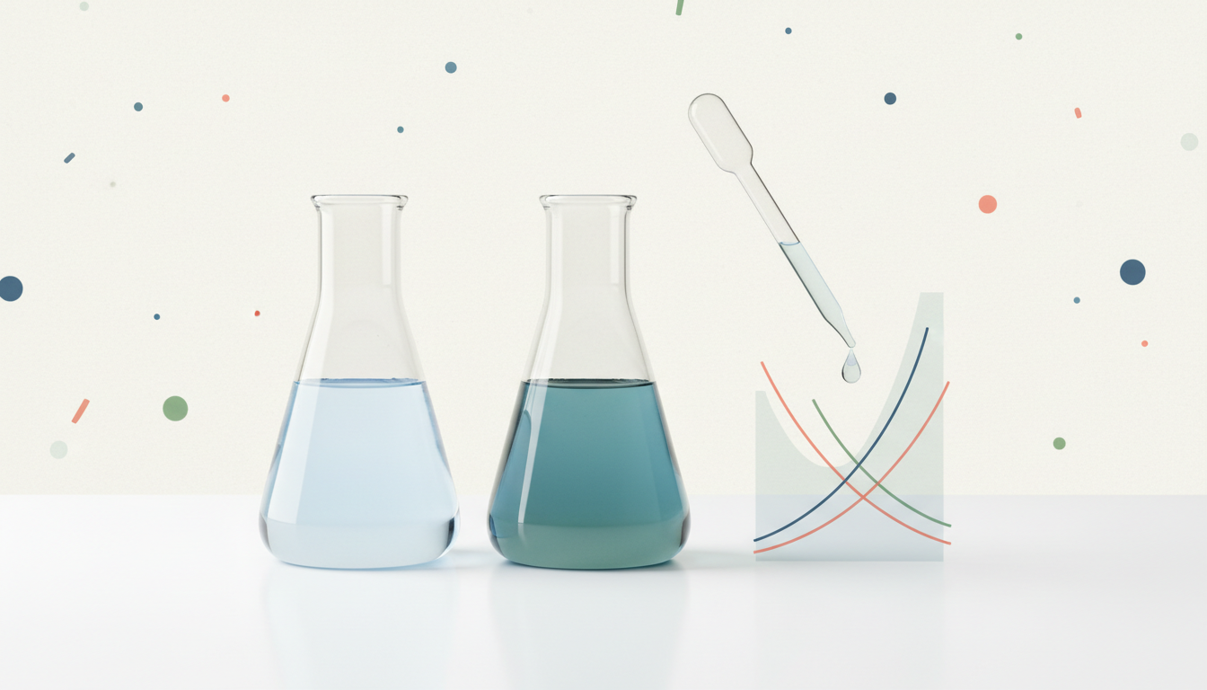
Two fictional weak-acid buffers can both have calculated starting pH 7.00 without having equal ability to resist added strong acid. One buffer contains five millimoles each of weak acid and conjugate base in a litre; another contains fifty millimoles of each.
Their starting conjugate-base-to-acid ratios are equal, so the ideal Henderson–Hasselbalch approximation gives the same initial pH when pKₐ is defined as seven. Their absolute amounts differ by tenfold.
Under a fixed theoretical addition of four millimoles of strong acid, the dilute solution consumes most of its available conjugate base while the concentrated solution consumes only a small fraction. Their computed final pH values therefore separate widely.
The exercise uses idealised solution chemistry, no volume change and fixed equilibrium parameters. It is not an instruction to prepare or test unverified chemicals, and the numbers are not real laboratory measurements.
pH is related to hydrogen-ion activity and describes an equilibrium state under chosen temperature and measurement conditions. Buffer capacity is about how much strong acid or base the solution can absorb before its pH shifts substantially.
A simple buffer consists of a weak acid HA and its conjugate base A⁻. The weak-acid pair can redistribute species when protons are added or removed, moderating the resulting acidity shift while useful reserve remains.
These two properties are not synonyms. A pH value may be reported precisely without giving the total moles of buffering species in a litre. Without those amounts, the response to a future addition remains unresolved.
The Gold Standard of Chemistry guide to hydrogen-ion activity explains why a measured pH also needs caution when interpreted as a direct concentration.
In the hypothetical dilute Buffer D, 1.000 L contains 0.005 mol HA and 0.005 mol A⁻. Its total formal buffer concentration is 0.010 mol/L. The initial two species each account for half that formal amount.
In the concentrated Buffer C, the same nominal volume contains 0.050 mol HA and 0.050 mol A⁻, giving 0.100 mol/L total formal concentration. C contains ten times the moles of each species.
Assume both use the same chemical conjugate pair with pKₐ=7.00, at compatible temperature. Ignore secondary reactions and activity differences in the first ideal calculation so the effect of the amounts is isolated.
The numbers are formal component balances, not a suggested real experimental recipe. Real pH requires the appropriate activity model and electrode calibration.
The approximate Henderson–Hasselbalch relation is pH=pKₐ+log₁₀([A⁻]/[HA]), where the ratio can also be expressed in the relevant formal mole amounts if they share one volume.
For D, the starting ratio is 0.005/0.005=1. For C, it is 0.050/0.050=1. Thus both give pH=7+log₁₀1=7 in the ideal model.
The mathematical equality is genuine, but it constrains only the ratio rather than the total quantity of the weak-acid pair. There are many possible formal concentrations consistent with a one-to-one ratio.
The Chemistry LibreTexts discussion of practical buffers distinguishes pH-setting ratios from concentration-dependent buffer performance.
Introduce an idealised 0.004 mol strong-acid addition to each nominal litre without changing its volume. Within the formal weak-acid buffer model, the reaction A⁻+H⁺→HA converts 0.004 mol of conjugate base into 0.004 mol of weak acid.
Thus the remaining base amount is its initial value minus 0.004, and the weak-acid amount is its initial value plus 0.004, provided the base remains positive and the ideal approximation applies.
The total HA+A⁻ formal amount is conserved under this simple conversion, because buffering species have changed form rather than disappeared.
A real reagent addition changes solution conditions and may introduce ionic-strength and dilution effects. Our controlled mathematical setup deliberately sets them aside.
Buffer D began with 0.005 mol A⁻ and 0.005 mol HA. After the theoretical reaction it contains 0.001 mol base and 0.009 mol acid.
The resulting ratio is 0.001/0.009=1/9, so pH_D≈7+log₁₀(1/9)≈6.045757. The theoretical decrease from the initial pH is about 0.954243 unit.
Four millimoles used eighty percent of the initial five-millimole conjugate-base reserve. The remaining base fraction is small, and the buffer now lies much closer to the end of its useful ratio range.
This is a calculated example, not a measured pH to six-decimal accuracy. It demonstrates the consequence of depleting a finite reserve while keeping the starting ratio fixed.
Buffer C begins with 0.050 mol of each species. Under the same conversion, it ends with 0.046 mol A⁻ and 0.054 mol HA.
The new ratio is 46/54≈0.851852, giving pH_C≈7+log₁₀(46/54)≈6.930364. Its theoretical pH decrease is only about 0.0696 unit.
Four millimoles consumed just eight percent of C’s starting conjugate-base moles. The small relative depletion preserves a ratio much closer to one.
Both solutions initially had pH seven and both received the same hypothetical acid amount. The different results arise from their total buffer species, not from a different initial conjugate-pair ratio.
In the same idealised model, a strong base converts HA to A⁻ through HA+OH⁻→A⁻+H₂O. This reverses the mole changes of an equal strong-acid addition.
Adding 0.004 mol formal strong base to D leaves 0.001 mol HA and 0.009 mol A⁻, giving pH≈7+log₁₀9≈7.954243. In C the corresponding amounts are 0.046 mol HA and 0.054 mol A⁻, giving pH≈7.069636.
The ideal numerical responses are symmetric around the starting pH because the starting amounts were equal and the stipulated perturbations reverse the same reaction.
Real laboratory solutions may not show perfect symmetry because activities, ionic strength, solvent chemistry or additional acid–base equilibria affect the measured result.
| Formal property | Dilute D | Concentrated C |
|---|---|---|
| Nominal volume | 1.000 L | 1.000 L |
| Initial HA and A⁻ | 0.005 mol each | 0.050 mol each |
| Total buffer concentration | 0.010 M | 0.100 M |
| Initial ideal pH | 7.000 | 7.000 |
| Acid added | 0.004 mol | 0.004 mol |
| Final HA | 0.009 mol | 0.054 mol |
| Final A⁻ | 0.001 mol | 0.046 mol |
| Final ideal pH | 6.0458 | 6.9304 |
An ideal weak-acid pair has an approximate differential buffer capacity contribution β≈2.303 C Kₐ[H⁺]/(Kₐ+[H⁺])², where C is the total formal molar concentration of the pair.
At pH=pKₐ, the expression simplifies to β≈(2.303/4)C≈0.57575 C, in mol L⁻¹ per pH unit under the stated ideal model.
D has C=0.010, yielding β≈0.0057575. C has C=0.100, yielding β≈0.057575. The concentrated model has ten times the local buffer capacity at the same starting conjugate ratio.
The Chemistry LibreTexts treatment of buffer capacity explains why the weak acid–base ratio and available amounts matter for pH resistance.
A local differential capacity describes sensitivity near the starting composition. For a small addition Δn in volume V, a first-order estimate is ΔpH≈−Δn/(βV) when activity assumptions and β variation are sufficiently controlled.
With Δn=0.004 mol and V=1 L, the concentrated initial β predicts ΔpH≈−0.0695, close to the exact finite-ratio model. Its perturbation changed the ratio only modestly.
For D the same initial slope predicts about −0.6947, but the finite-ratio shift is about −0.9542. The derivative is no longer a good constant approximation over such a large depletion.
A reliable calculation distinguishes initial capacity from an entire titration curve. When a large fraction of one buffer component is consumed, re-evaluate the chemical composition rather than relying on the original slope.
Start from equal conjugate amounts n₀ for HA and A⁻. To move down one ideal pH unit, the final base-to-acid ratio must become 0.1. Let δ be the strong-acid amount converted under the model.
Set (n₀−δ)/(n₀+δ)=0.1. Rearranging gives n₀−δ=0.1n₀+0.1δ, so δ=(9/11)n₀.
For D, n₀=0.005 mol, giving δ≈0.0040909 mol. For C, n₀=0.050, giving δ≈0.040909 mol. The latter formal addition is tenfold larger for the same one-unit model change.
These are analytical ratios, not a practical titration procedure or a universal buffer-capacity definition. A chemical system needs its own validated equilibrium conditions.
Adding 0.005 mol strong acid to D would consume its initial 0.005 mol conjugate base in the simple stoichiometric balance. The calculated final base amount reaches zero, and log([A⁻]/[HA]) is not suitable for predicting a finite pH.
The Henderson–Hasselbalch relation is an approximation involving appreciable conjugate species and suitable acid-base equilibrium conditions. Near exhaustion, additional free acid and weak-acid dissociation need fuller treatment.
A complete real calculation may require mass balance, charge balance, equilibrium constants and activity effects. Substituting zero or negative concentrations into the logarithm is not a valid continuation of the initial buffer calculation.
The Chemistry LibreTexts buffers chapter describes the limited useful range of conjugate-pair buffering.
The exact equality of the initial calculated pH values is based on an ideal approximation. Real pH refers to hydrogen-ion activity, and the activity coefficients in a concentrated solution can differ from those in a dilute solution.
Weak-acid dissociation constants depend on temperature. Electrode calibration, junction potentials and additional ions can change apparent pH readings. One cannot infer identical measured pH solely from equal formal HA/A⁻ ratios under arbitrary experimental conditions.
Our theoretical model holds chemistry, temperature and volume fixed to isolate concentration as a cause of different buffering response. Practical work must check whether that model is appropriate for the solution and intended decision.
A readout with two decimals is not a guarantee of matching acid reserve or measurement accuracy. The chemistry and calibration need to be documented separately.
Does identical pH guarantee identical buffer capacity? No. The initial ratio can be the same when formal amounts differ by tenfold, giving very different responses to a fixed addition.
If the added acid amount were only 0.001 mol, D would have 0.004 mol A⁻ and 0.006 mol HA, while C would have 0.049 and 0.051. Calculate both pH values and compare with the four-millimole results.
If both starting components in D are doubled without changing their ratio, the ideal initial pH stays seven while the finite resistance to added acid increases. The new amounts—not the initial ratio—explain the change.
For another practice problem, find the formal strong-base amount required to raise the ideal pH by half a unit. Check that both conjugate species remain positive in your proposed solution.
The main result is that initial pH does not determine how much acid or base a solution can neutralise. D and C have the same ideal starting pH, but the four-millimole theoretical addition produces pH values near 6.046 and 6.930.
Read The Gold Standard of Chemistry, Enzyme pH Profiles and Buffer Effects, and the practical chemistry discussion of buffer choice for related principles.
The two concentrations, ideal pKₐ and finite additions are original hypothetical teaching values. They are not experimental findings or specific material recommendations.
Continue via the Gold Standard hub. A trustworthy pH comparison identifies both the equilibrium state and the chemical reserve available when conditions change.
Advanced worked companion: finite pH changes and buffer reserve
1. Prove the finite-addition equation rather than memorising a number
Let the initial formal mole amounts of weak acid and conjugate base be a₀ and b₀, both positive. Add a formal amount δ of strong acid under the assumption that it converts available A⁻ into HA in the same well-mixed nominal volume. The new mole amounts are a=a₀+δ and b=b₀−δ. Conservation of the buffer pair is apparent: a+b=a₀+b₀.
Under a suitable Henderson–Hasselbalch approximation, the final pH is pKₐ+log₁₀[(b₀−δ)/(a₀+δ)]. The starting pH is pKₐ+log₁₀(b₀/a₀). Identical starting ratios do not force identical final ratios, because a fixed δ may be a large fraction of one buffer and a small fraction of another.
For equal initial amounts a₀=b₀=n₀, define fractional depletion f=δ/n₀. Then pH−pKₐ=log₁₀[(1−f)/(1+f)]. The dimensionless fraction f controls the ideal change. Buffer D has f=0.8 after the 4 mmol addition, while C has f=0.08. That difference precisely explains the two calculated final pH values.
The mathematical domain matters. For positive final base and acid amounts, −1 For D, f=0.004/0.005=0.8, so the final ratio is (1−0.8)/(1+0.8)=0.2/1.8=1/9. The theoretical pH is 7+log₁₀(1/9)≈6.045757. This gives a pH departure of approximately -0.954243. For C, f=0.004/0.050=0.08, so its final ratio is 0.92/1.08=46/54. The resulting theoretical pH is approximately 6.930364, with departure -0.069636. The same reaction model, pKₐ and added amount were used for both. The ratio method and the explicit mole tables are independent routes to the same numerical outputs. When two calculations disagree, inspect the denominator, conversion direction and units. A common error is to subtract the strong-acid amount from HA rather than from A⁻, reversing the chemistry of protonation. The exact decimal outputs are arithmetic aids within an ideal model. They are not claims that an ordinary pH electrode or a real solution is accurate to six places. The proper number of reported digits in an experimental result depends on calibration and input uncertainty. Repeat the calculation with only 0.001 mol of strong acid in each theoretical litre. Buffer D then has 0.004 mol A⁻ and 0.006 mol HA, so pH≈7+log₁₀(2/3)≈6.823909. Buffer C has 0.049 mol A⁻ and 0.051 mol HA, giving pH≈6.982626. Both solutions move closer to pH seven than they did after the four-millimole addition, but the concentrated solution still exhibits the smaller shift. The nominal pH drops are about 0.1761 and 0.0174 units respectively. At the formal level, all the buffer pairs still sum to their initial totals. D’s new HA+A⁻ total is 0.010 mol; C’s remains 0.100 mol. That conservation is a valuable check before any equilibrium calculation is considered. An observed response in real chemistry might not follow these simple figures because ionic activity, dilution and additional equilibria can change with the addition. The exercise isolates a constrained stoichiometric principle, and each conclusion should remain attached to those constraints. Suppose a hypothetical decision allows a downward pH change of at most 0.5 unit in the model. Starting from pH=pKₐ, the final ideal base-to-acid ratio at the boundary is q=10^(−0.5)≈0.316228. Set (n₀−δ)/(n₀+δ)=q and solve for δ. Rearrangement gives δ/n₀=(1−q)/(1+q)≈0.519494. Thus D’s formal 0.5-unit addition threshold is approximately 2.5975 mmol, and C’s is approximately 25.9747 mmol. C again supports tenfold the amount under this fixed ratio and volume model. This algebra clarifies what a capacity comparison must specify. ‘Resists pH change’ means little without naming an added amount, volume, direction and permitted change. Comparing buffers at different volumes without normalising the quantities would also be misleading. The same idea can be used for an upward change by considering conversion of HA into A⁻ by base. The formal symmetry of our equal-ratio initial condition does not imply every real multi-component buffer responds symmetrically, because activities and side reactions may differ. For equal starting species n₀ and f=δ/n₀, pH−pKₐ=log₁₀[(1−f)/(1+f)]. Differentiate this expression with respect to f: d(pH)/df=−2/[ln10×(1−f²)]. At f=0, the initial slope is −2/ln10≈−0.868589 pH unit per unit fractional addition. Because the formal amount δ equals f n₀ and the total concentration C equals 2n₀/V, the initial amount per unit pH change becomes β≈(ln10/4)C≈0.575646C in mol L⁻¹ per pH unit under the same ideal model. This independently derives the proportionality to total buffer concentration. The corresponding β values are about 0.0057565 and 0.057565 mol L⁻¹ per pH unit for D and C. A textbook using 2.303 instead of the unrounded ln10 obtains extremely similar numbers. The difference is presentation precision rather than a chemical distinction. The slope does not remain fixed as f approaches one; the formula itself shows a denominator 1−f². This is why a small local buffer-capacity estimate can understate a large finite pH excursion as conjugate base is depleted. At the starting composition, a linearised estimate for a small strong-acid addition is ΔpH≈−Δn/(βV). For C and the four-millimole example this gives a shift around −0.0695 pH unit, close to the finite-ratio result around −0.0696 because the conjugate ratio remains near one. For D, the same local approximation gives about −0.6949 pH unit, whereas the finite-ratio result is −0.9542. This discrepancy is meaningful: the dilute buffer traverses a much larger portion of its titration curve. The initial derivative cannot be extrapolated as a constant over the entire interval. Near depletion, a complete model may need to include the weak-acid equilibrium and the free strong-acid contribution. Continuing to use a formula that requires both HA and A⁻ as appreciable equilibrium species after one has formally vanished is not sound chemistry. An analyst should therefore decide between a local differential estimate and a finite perturbation calculation according to the size of the change. The reported uncertainty also grows when activity coefficients, volume changes and side reactions have not been measured. A fixed buffer pH can be approached by choosing a conjugate pair with a suitable pKₐ and an acid/base ratio. Once that ratio is determined, total formal concentration helps set how much perturbation can be accommodated before the ratio changes substantially. At pH=pKₐ, the equal-ratio model is centred near the usual maximum chemical buffer capacity for the single weak-acid contribution. At pH one unit above pKₐ, the ideal ratio is ten to one, with relatively little HA reserve for added strong base. In the simplified single-pair formula β=(ln10)C·r/(1+r)², where r=[A⁻]/[HA], the factor r/(1+r)² equals 1/4 at r=1 but only 10/121≈0.08264 at r=10. Even for equal C, the local capacity is substantially lower in the more skewed conjugate composition. This creates an additional kind of non-uniqueness: two solutions with the same pH and total concentration can still have different capacity if their buffer systems have different pKₐ values and corresponding acid/base ratios. Chemical identity is part of the information required. If a suitable ideal buffer is diluted so both HA and A⁻ concentrations fall by the same factor, their formal ratio is unchanged. Henderson–Hasselbalch therefore predicts the same starting pH within its assumptions, even though the total concentration and local buffer capacity per unit volume decrease. That is the conceptual relationship between D and C, although our exercise constructed them directly rather than instructing a real dilution. A fixed acid addition per litre consumes a larger fraction of the dilute buffer’s base reserve and produces a greater formal pH response. At sufficiently low concentrations, water autoionisation, activity changes and other equilibria can matter enough to spoil the simple ratio prediction. Chemistry LibreTexts’ Henderson–Hasselbalch analysis discusses why an ideal approximation cannot be extended indefinitely into extreme dilution. Neither the initial ratio nor a neat textbook calculation replaces a properly calibrated pH measurement and chemical-speciation assessment when a real application requires accuracy. Buffer D’s starting conjugate-base amount is 0.005 mol. If the formal strong-acid addition reaches that same 0.005 mol amount, the simple reaction ledger gives zero A⁻ and 0.010 mol HA. Attempting to calculate pH through log₁₀(0/0.010) is not a useful physical result. At this endpoint the system is no longer represented as a balanced buffer pair in the stated form. Additional equilibrium equations are required to estimate the actual hydrogen-ion activity and determine how much the weak acid dissociates. Excess strong acid after that point changes the calculation again. The endpoint is not an experimental recommendation. Real reagent additions require validated conditions and appropriate safety practices, and the present theoretical variables do not identify a chemical substance with a known handling protocol. This failure mode teaches a general analytical principle: a mathematical approximation may give helpful predictions inside a stated domain but should not be treated as exact beyond the point where its defining assumptions cease to hold. An evidence-based buffer report identifies the weak-acid species, formal conjugate amounts, relevant pKₐ at measurement temperature, nominal volume, additions and equilibrium assumptions. It also records any significant ionic-strength or activity corrections. Observed pH requires a calibrated measuring system and documented conditions. The reader should be able to distinguish formal calculated pH from a measured reading with its uncertainty. Six displayed decimal places in a teaching computation do not imply six-decimal pH metrology. To report buffering performance, specify whether the result is an initial differential β, a finite addition per litre for a chosen pH interval, or a titration curve. Those three descriptions relate to one another but are not interchangeable across large changes. Relevant sources are Physical Chemistry of Buffers and Practical Aspects of Buffers. The amounts in this article are original fictional teaching parameters.2. Check the four-millimole calculation using one shared ratio formula
3. Change just the acid quantity and watch the contrast evolve
4. Solve for a specified half-unit pH response
5. Reconstruct the local differential capacity from the general curve
6. Understand why initial local capacity is not a full titration forecast
7. Keep acid–base ratio and total concentration as separate design variables
8. What tenfold dilution does and does not preserve
9. A rigorous example of the endpoint where buffering assumptions fail
10. Audit a chemistry report without mistaking pH for capacity