
A river can keep flowing after a storm ends, but its hydrograph does not label every source of water. Hydrograph separation estimates contributions beneath the observed flow curve. It becomes useful when the reader can distinguish the measured total from the assumptions used to divide it.
This guide builds two contrasting separations from one original dataset, calculates their volumes, and shows how a chemical mixing check depends on its own conditions. It continues the Hydrology subject guide with a focused evidence question: what does an estimated baseflow component actually establish?
Choose the question you need
eduKateSG · Hydrology · A focused guide with worked examples and independent checks.
Understand the evidence · Chapters 1–3. Observed discharge, pathways and a bounded dataset.
Calculate and challenge the estimate · Chapters 4–6. Volumes, sensitivity and a mixing example.
Transfer into better questions · Chapters 7–10. Data quality, unequal intervals, use and limitations.
Full chapter index · Hydrology subject guide · Learning that transfers into life
Chapter contents
Understand the evidence · Chapters 1–3
Calculate and challenge the estimate · Chapters 4–6
CHAPTER 1 OF 10 · Understand the evidence
1. Separate the measured curve from the inferred components
A discharge hydrograph records how the estimated volume rate at a river section changes through time. A separation divides that record into components according to a model. The original curve and the separated curves therefore have different evidential roles.
In a two-component notation, Q = B + R, where Q is total discharge, B is estimated baseflow and R is the remaining, faster-response component. The identity tells us that R = Q − B. It does not tell us which B is physically correct.
The USGS HYSEP report describes several separation methods using daily mean discharge. The existence of several methods matters: a smooth lower line can be an algorithmic interpretation rather than an independently observed groundwater flow.
Before calculating anything, label each curve measured or estimated and state the time interval. A learner who sees three polished lines on one chart should still know which information came from a gauge and which came from an analytical choice.
CHAPTER 2 OF 10 · Understand the evidence
2. Explain slower pathways without turning speed into water age
Baseflow commonly describes the contribution sustaining streamflow between precipitation events through delayed pathways, often associated with groundwater. Quickflow names the remainder in the chosen separation. These definitions help organise a response, but they do not automatically identify the age or exact travel route of every water molecule.
The USGS study of chemically constrained separation sets out its conceptual model and limitations. Read those conditions alongside the result, especially where multiple sources contribute.
Imagine rainfall increases pressure and connectivity within a catchment. Water already stored there may reach the channel during the rising limb. A rapid increase in flow does not, by timing alone, prove that all additional water fell in the latest shower.
For students, keep three questions distinct: how quickly did discharge respond, which pathway contributed, and when did the water enter the system? A hydrograph directly helps with the first. Answering the others needs additional evidence and a suitable model.
Consider a fictional five-hour record. For arithmetic clarity, treat each value as the constant discharge throughout one complete hour, not as a point measurement that needs interpolation. The rates are in cubic metres per second. Each interval therefore lasts 3,600 seconds.
Two possible classroom separations are supplied. Model A keeps baseflow at 2 m³/s. Model B allows it to rise and then recede. Neither was fitted to a real stream. Their purpose is to show what changes when the partition assumption changes while the observed total is held fixed.
Check both candidates before integrating. Every proposed B is non-negative and no greater than Q, so neither produces a negative remainder. That is a necessary arithmetic check here; it is not sufficient proof that either represents the actual catchment.
Do not call these hourly values daily means, and do not insert a six-hour interval by treating five rows as five gaps between endpoints. The meaning of a row determines the calculation.
| One-hour interval | Total Q, m³/s | Baseflow A, m³/s | Baseflow B, m³/s |
|---|---|---|---|
| 1 | 2 | 2 | 2 |
| 2 | 8 | 2 | 2.5 |
| 3 | 12 | 2 | 3 |
| 4 | 7 | 2 | 2.8 |
| 5 | 3 | 2 | 2.4 |
CHAPTER 4 OF 10 · Calculate and challenge the estimate
4. Convert the rates into volumes
First calculate total volume. The sum of the five interval rates is 2 + 8 + 12 + 7 + 3 = 32. Because each applies for the same 3,600-second interval, total volume is 32 × 3,600 = 115,200 m³.
Model A assigns 2 × 5 × 3,600 = 36,000 m³ to baseflow. The remainder is 115,200 − 36,000 = 79,200 m³. Its period baseflow index, defined here as baseflow volume divided by total volume, is 36,000/115,200 = 0.3125, or 31.25%.
Model B has a baseflow-rate sum of 2 + 2.5 + 3 + 2.8 + 2.4 = 12.7. Its assigned baseflow volume is 45,720 m³, leaving 69,480 m³ in the remainder. Its index is 45,720/115,200 = 0.396875, about 39.7%.
The observed total has not changed. The allocation differs by 9,720 m³. Reporting only a rounded percentage would conceal both the underlying volume and the dependence on the selected model. A complete answer retains the rates, interval lengths, definition and assumed partition.
CHAPTER 5 OF 10 · Calculate and challenge the estimate
5. Use disagreement as a sensitivity check
The two indices do not form a statistical confidence interval. We selected two illustrative models; we did not establish a probability distribution for all plausible separations. Calling the range 31.25–39.7% a 95% interval would invent information.
Instead, use the difference to identify a decision-sensitive assumption. If a proposed conclusion depends on the baseflow contribution being below 35%, the choice between these two models matters. If the question is only total transported volume, the partition is irrelevant to that calculation.
The USGS comparison of separation methods reports differences between methods and discusses assumptions. That motivates inspecting method choice; it does not validate our two invented lines.
Ask which observation could constrain the uncertainty. Relevant hydrogeological information, recession behaviour, suitable tracers or additional measurements may help. Simply selecting the smoother line is not an independent test. The stronger explanation states which part of the result is robust and which depends on the partition.
CHAPTER 6 OF 10 · Calculate and challenge the estimate
6. Try a chemical mixing check with explicit conditions
A fictional instantaneous observation has stream discharge 9 m³/s and tracer concentration 200 units. Assume two endmembers: baseflow at 400 units and quickflow at 100 units. Assume the tracer mixes conservatively, the endmembers are representative, and no third source matters at the observation.
Write the mass balance: 9 × 200 = B × 400 + (9 − B) × 100. Expanding gives 1,800 = 400B + 900 − 100B, so 900 = 300B and B = 3 m³/s. The baseflow fraction is one third.
Now change only the assumed baseflow endmember to 300 units. The fraction becomes (200 − 100)/(300 − 100) = one half, so B = 4.5 m³/s. The same stream measurement now gives a different allocation because an input assumption changed.
This is a model check, not a ready-to-use field protocol. A tracer that reacts, varying endmembers or multiple contributing sources can invalidate the two-component interpretation. The USGS chemical-mass-balance study makes these model limitations part of its analysis.
CHAPTER 7 OF 10 · Transfer into better questions
7. Inspect missing records, time resolution and regulation
A missing high-flow interval changes the denominator in a baseflow index. If an instrument fails at the peak and the analyst sums only the remaining intervals, the final fraction may look more precise than the record deserves. Missing is not zero.
Time resolution also matters. A daily mean can support a daily-volume calculation while concealing a short peak. A separation calibrated for one resolution should not silently be applied to another as though the input series were unchanged.
Reservoir releases, abstractions, diversions and other controls can add patterns that a simple natural-catchment explanation misses. An algorithm may still draw a smooth line. The existence of an output does not establish that the assumptions fit the site.
Use a small data checklist: gauge location, units, interval definition, record gaps, changes in measurement, known controls, method and parameter version. The USGS Groundwater Toolbox guide situates hydrograph methods within a wider set of analyses. A separation is one contribution to that work, not a substitute for understanding the system.
CHAPTER 8 OF 10 · Transfer into better questions
8. Transfer the calculation to unequal intervals
A new fictional record has Q = 4 m³/s for 30 minutes and Q = 2 m³/s for 90 minutes. A supplied model assigns B = 1 m³/s during both intervals. Find the total volume, baseflow volume and index.
The total is 4 × 1,800 + 2 × 5,400 = 18,000 m³. The baseflow volume is 1 × (1,800 + 5,400) = 7,200 m³. The index is 7,200/18,000 = 40%.
Why not average the instantaneous fractions 1/4 and 1/2 to obtain 37.5%? That would give the two observations equal weight despite different durations and total volumes. Even a duration-weighted average of the fractions is not generally the required volume ratio. Compute the two volumes first.
Now remove the model and retain only Q. Can you calculate the same baseflow index uniquely? No. Total discharge determines total transported volume under the interval assumptions, but it does not by itself identify the component volumes. This is the central evidence limit of separation.
CHAPTER 9 OF 10 · Transfer into better questions
9. Connect the partition to a real question
For a water-quality question, the quantity of interest might be the load carried under different flow conditions. For a water-resource question, it might be persistence between rainfall events. Neither is answered completely by a single baseflow percentage.
Two sites could share the same index while having different absolute flows, seasons and regulation. A high proportion of a very small total is not necessarily a large resource. A low-flow ecological question may depend on duration and timing that a whole-period index compresses.
Before adding more calculations, write the intended claim: what does the estimated component explain, over which period, and what independent check would support it? Then choose the method appropriate to that question.
For learning, ask the student to defend one statement and reject one overstatement. “Model B assigns 45,720 m³ to baseflow” follows from the example. “Exactly that volume entered the river from groundwater” needs evidence the example does not supply. Keeping those sentences distinct is scientific progress.
CHAPTER 10 OF 10 · Transfer into better questions
10. Questions about baseflow and hydrograph separation
Is baseflow measured directly by drawing the lower line? No. The line is an estimate from the selected method. Additional observations can help constrain or test it.
Is quickflow always new rain travelling over the ground? No. A response-based partition does not by itself establish water age or a unique pathway.
Can the estimated component exceed total flow? Not in the non-negative two-component model used here. Such an output would require checking the method or interpretation rather than accepting a negative remainder.
Does a higher baseflow index prove a healthier river? No. The index describes a modelled proportion over a stated record. River condition involves other quantities, timing, quality and ecological evidence.
Which calculation should a beginner master first? Convert rates and durations into volumes, then verify that the component volumes add to the total. Add interpretation only after units and boundaries are stable.
What is the next useful action? Choose a supplied record, label measured and inferred quantities, state the interval convention and compare one alternative partition. Explain the conclusion that changes and the conclusion that remains.
Continue through the connected guides
Understand the water pathways
Hydrogeological Engineering: groundwater pathways with evidence develops subsurface investigation. How Science Works: Hydrology sets out the wider catchment system.
Connect quantity, quality and use
Water quality monitoring follows what observations can establish. Environmental laboratory testing: representative samples and clear limits examines the measurement chain. Water Resources Engineering: catchment to community connects estimates with planning.
Compare a connected question
Distinguish source partitioning from frequency and chronology in The Gold Standard of Hydrology | Flow-Duration Curves and the Drought Sequences They Hide.
Sources and scope
Methods and conceptual limits: Sloto and Crouse, HYSEP (USGS, 1996); Raffensperger and colleagues, chemically constrained hydrograph separation (USGS, 2017); USGS Groundwater Toolbox guide (2015).
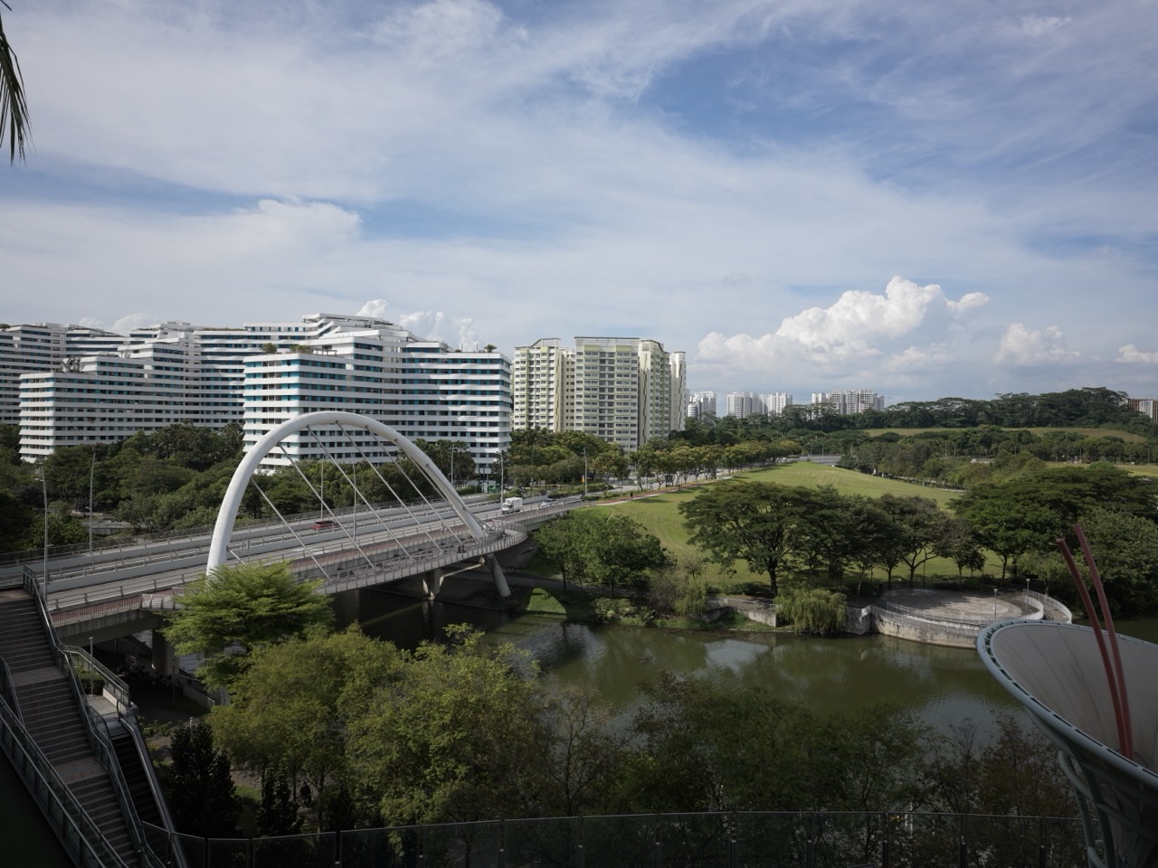
The photograph shows a canal and bridge at Punggol Waterway Park. It illustrates an urban water setting; the numerical examples do not describe that waterway. The two partitions and tracer values here are invented to expose the accounting and assumptions. They are not recommended parameters, a validated site model, a groundwater-resource assessment or an operational flood forecast.
The numerical datasets and classroom scenarios in this guide are invented teaching examples. Sources and linked reading were checked on 21 October 2026. “Gold standard” describes the educational benchmark explained here; it is not an accreditation.
Hydrology root guide · The Gold Standard of Education · Explore How X Works