
Find the question you need
The chapter text stays open. Choose a route or use the five expandable chapter groups below.
Define the actual question · Construct two stationary sources · Calculate uncertainty and dependence · Use the result responsibly · Practice and connected reading
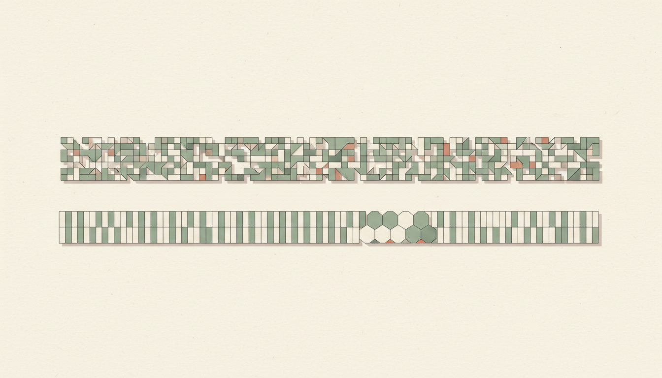
Two streams can each contain zero and one with equal probability, yet behave very differently when you read them in order. Here is how a persistent Markov process creates less uncertainty per new symbol than independent fair bits—even though their one-symbol entropies agree.
Chapter index
Define the actual question · Chapters 1–2
1. Why a fair zero–one count can hide predictable sequences · 2. Calculate the one-symbol entropy shared by both sources
Construct two stationary sources · Chapters 3–5
3. Construct Source A: independent fair symbols · 4. Construct Source B: a symmetric persistent Markov chain · 5. Prove stationarity and compare the conditional chances
Calculate uncertainty and dependence · Chapters 6–9
6. Calculate the entropy rate of the persistent chain · 7. See the difference across ten-symbol blocks · 8. Measure persistence without confusing it with certainty · 9. Relate entropy reduction to information in the past
Use the result responsibly · Chapters 10–10
10. Understand what this means—and does not mean—for compression
Practice and connected reading · Chapters 11–12
11. Frequently asked questions and two counterexamples · 12. Connect the mechanism to Probability and Information Theory
Suppose two fictional data sources each output a stream of zeroes and ones. On every individual time step, each source has a 50% probability of outputting zero and a 50% probability of outputting one. If we observe just one symbol without information about earlier symbols, both sources are equally uncertain.
Now ask a different question: after reading yesterday’s symbol, how difficult is it to predict tomorrow’s? Source A draws each symbol independently, like repeated fair coin flips. Source B usually repeats its previous symbol, changing only occasionally. The individual zero–one probabilities are the same, but the sequence structures are not.
Information theory distinguishes uncertainty in a single random symbol from the uncertainty generated by an entire stochastic process. The former is captured by a marginal entropy; the latter, when properly defined, is captured by an entropy rate. A model that reports just one histogram can miss a substantial part of the second question.
This lesson uses exact invented stochastic models, not an extracted computer log or a measurement of a real language. We will specify the mechanisms, derive their stationary distributions, calculate both entropies, and explain what a compression claim would actually require.
Let Xt be either 0 or 1. For a binary random variable with probability p of one, the Shannon entropy in bits is h₂(p) = −p log₂p − (1−p)log₂(1−p), with the usual convention that zero-probability terms contribute zero.
For p=1/2, the result is −(1/2)(−1)−(1/2)(−1)=1 bit. That is the maximum entropy of a binary symbol with only these two possible values.
Both sources are constructed so that P(Xt=0)=P(Xt=1)=1/2 at every time t. They therefore share H(Xt)=1 bit. The equality is exact in the probability model; a finite realised sequence may contain 48% ones or 53% ones through sampling variability.
Calling this one-bit calculation ‘the information rate’ would be premature. It does not yet say what an observer already knows when the next symbol arrives, or whether successive outputs are related. To answer that, we must describe the joint process rather than only the one-symbol marginal.
Source A draws X₁, X₂, X₃, … independently with equal probability of zero and one each time. Knowing Xt gives no extra information about Xt+1. Conditional on any past history, the next symbol remains fair.
In this model, P(next=0 | current=0)=1/2 and P(next=1 | current=1)=1/2. The same holds when the current value is the opposite. Conditional entropy H(Xt+1|Xt) is consequently 1 bit.
For a block of n independent symbols, the joint entropy is n bits because independent entropies add. A block of ten symbols has ten bits of Shannon entropy, and the entropy generated per symbol is 1 bit in the long-run sense.
An individual ten-symbol output such as 0000000000 is not impossible under this model. It is just unusual. The fact that a sample looks patterned does not, by itself, prove that the underlying process was dependent. Model assumptions and repeated evidence matter.
Source B starts with a fair initial symbol: P(X₁=0)=P(X₁=1)=1/2. At each later step, it retains its current state with probability 0.9 and switches to the other state with probability 0.1. The switching decisions are independent of the past conditional on the current state.
The transition matrix has rows for the current state and columns for the next state. It is P = [[0.9,0.1],[0.1,0.9]]. Both rows sum to one, and its symmetry makes (1/2,1/2) a stationary distribution.
Starting in that stationary distribution matters. It ensures each time step remains marginally fair, despite the strong preference to stay in the same state. Without the specified initial distribution, early time-step marginals need not be exactly one-half even if the chain eventually approaches one-half.
This is a first-order Markov model: the current state contains all history information needed to compute the next-step probabilities under the model. It does not claim that real-world processes are always first order; that is a testable and sometimes questionable modelling choice.
Assume the distribution before a step is (0.5,0.5). The probability of next being zero is 0.5×0.9 + 0.5×0.1 = 0.5. The probability of next being one is 0.5×0.1 + 0.5×0.9 = 0.5. Thus a fair distribution stays fair after one step and therefore at every step by induction.
The one-symbol entropy stays at one bit. But knowing the previous value changes the next-step probabilities dramatically. After a zero, the chance of another zero is 90%; after a one, the chance of another one is also 90%. In Source A, the corresponding chances are each 50%.
Here is why equal marginal frequencies do not imply independent trials. A histogram discards ordering. It records how often symbols appear without retaining which pairs occurred consecutively. An ordered sequence can be highly dependent even when each possible symbol occupies half the stationary probability mass.
The general distinction complements the Gold Standard Probability example of equal marginals with different overlap rates. There the missing relationship is between two binary events; here it is between successive outputs of a stochastic process.
| Transition | Independent source A | Persistent source B |
|---|---|---|
| 0 → 0 | 0.5 | 0.9 |
| 0 → 1 | 0.5 | 0.1 |
| 1 → 0 | 0.5 | 0.1 |
| 1 → 1 | 0.5 | 0.9 |
| Stationary P(0), P(1) | 0.5, 0.5 | 0.5, 0.5 |
For a stationary first-order Markov chain, the entropy rate equals H(Xt+1|Xt). Under the symmetric transition rule, each conditional distribution is (0.9,0.1) in some order, so the answer is h₂(0.1).
Compute h₂(0.1)=−0.1log₂0.1−0.9log₂0.9≈0.468996 bits per symbol. This is less than one-half bit per new symbol even though the marginal entropy of each symbol is one full bit.
Compare Source A’s rate of 1.000000 bit/symbol with Source B’s approximately 0.469000. Their one-symbol probability tables agree exactly; their entropy rates differ by about 0.531 bit per symbol. That difference comes from the predictive value of the immediate past.
The MIT Information Theory lecture notes distinguish entropy, mutual information and entropy rate. The documented stationary Markov-chain entropy-rate formula evaluates the stationary-state-weighted conditional transition entropies. We use the same mathematics here with invented transitions.
The persistent chain can be generated by selecting a fair first bit and then using independent flip indicators F₁,F₂,…, each equal to one with probability 0.1. Let Xt+1=Xt XOR Ft. Given the first symbol, every later symbol is determined by the intervening flip choices.
This mapping between (X₁,F₁,…,Fn−1) and (X₁,…,Xn) is one-to-one. Therefore H(X₁,…,Xn)=1+(n−1)h₂(0.1). This is a finite-block identity, not merely a limiting approximation.
For a ten-symbol block, the persistent source has 1+9×0.468996≈5.22096 bits of joint entropy. Source A has exactly ten bits. Divide by ten: the persistent block average is about 0.52210 bit per symbol, still above its long-run rate because the first symbol needs a full bit.
As n increases, the one-time cost of the first bit becomes negligible and the block average tends to 0.468996. This explains why the entropy rate is not generally equal to the marginal entropy, and why short-file compression cannot be judged by a long-run theoretical number alone.
| Quantity | Independent A | Persistent B |
|---|---|---|
| Single-symbol entropy | 1 bit | 1 bit |
| Entropy rate | 1 bit/symbol | 0.468996 bit/symbol |
| Ten-symbol joint entropy | 10 bits | 5.22096 bits |
| Adjacent-symbol mutual information | 0 bit | 0.531004 bit |
Across a sequence of 101 symbols there are 100 successive transitions. For Source A, the expected number of changes is 100×0.5=50. For Source B, it is 100×0.1=10. Those are expectations; a particular run need not contain exactly those counts.
The probability of ten consecutive no-change transitions is 0.9¹⁰≈0.3487 for Source B but 0.5¹⁰≈0.0009766 for Source A, if the starting symbol is not constrained beyond each source’s own model. Long runs are therefore much more common under the persistent process.
Yet 90% persistence is not perfect predictability. Each next symbol still has a ten-per-cent chance to switch, and an arbitrarily long period without a switch does not reduce the model’s next-step switch probability below 0.1. That would require a different process, for example one with hidden changing regimes.
When presenting patterns, distinguish expected behaviour, exact event probabilities and realised frequencies. One unusually long sequence should prompt investigation, not a declaration that the underlying entropy rate has been measured exactly.
Mutual information between adjacent symbols is I(Xt;Xt+1) = H(Xt+1)−H(Xt+1|Xt). In Source B, that equals 1−0.468996≈0.531004 bits.
In Source A, the corresponding mutual information is zero. This makes the comparison intuitive: the persistent source’s immediately previous bit provides useful predictive information, while the independent source’s previous bit provides none.
The term ‘0.531 bits of mutual information’ is an average over the stipulated probability distribution. It is not a claim that every actual pair of symbols literally carries the same amount of useful evidence. Different observed transitions can have different information contributions.
Information theory offers multiple measurements for different questions. Marginal entropy summarises uncertainty in a single variable; mutual information evaluates statistical dependence; entropy rate measures the average uncertainty of new symbols in a process. A report should choose the quantity its practical inference requires.
A persistent source creates repeated patterns that a suitable compressor may exploit. In an ideal long-run lossless-coding setting with known or learnable stationary source statistics, entropy rate represents a fundamental average description-length benchmark in bits per symbol.
That is not a promise that a ten-byte file will be compressed to 4.69 bits, or that every individual realisation achieves the same length. Real codes have headers, finite-block overhead, implementation constraints and model mismatch. A particular short sequence may compress unusually well or poorly.
If a compressor assumes independent fair bits, it has no reason to exploit run persistence. If it models transition probabilities effectively, it can describe the initial state and subsequent switches more efficiently in the long run. This is a model-based opportunity, not guaranteed performance of a named coding algorithm.
Readers can continue with The Gold Standard of Coding Theory to separate source representation, redundancy, error correction and operational coding constraints. A predictive description and a reliable transmission system solve related but different engineering problems.
Does one bit of entropy per symbol mean independent symbols? No. Each symbol of the persistent chain has one bit of marginal entropy, while transitions carry dependence and the entropy rate is lower.
Can two processes with the same entropy rate behave differently? Yes. Change the Markov switch probability from 0.1 to 0.9 while preserving the fair stationary distribution. Because h₂(0.9)=h₂(0.1), the rate stays about 0.469 bits per symbol, but the process now usually alternates instead of usually repeating. Entropy rate alone does not identify the full transition behaviour.
What if the switch probability is 0.5? The symmetric chain becomes independent fair symbols, with entropy rate h₂(0.5)=1 bit per symbol. Both the marginal entropy and entropy rate match Source A.
What if the process starts in state zero for certain? Then its first-symbol entropy is zero and early marginals are not fair. With a 0.1 switching rule the long-run stationary rate remains the same under standard assumptions, but the exact finite-block identity based on a fair first bit must be changed.
Practice: for p=0.01, compute h₂(0.01)≈0.08079 bit per transition. Explain why stronger persistence makes a new symbol more predictable even while the stationary zero–one split remains fifty–fifty.
The conclusion is about the question, not the attractiveness of one statistic. Two sources can have the same marginal distribution and still differ profoundly in conditional prediction, sequence lengths and entropy rate. Any statement about compressibility or dependencies must specify the process model and observation history.
Return to The Gold Standard of Information Theory for the subject foundation. Follow Fixed Marginals, Different Overlap Rates and Reinforced Urns and Dependent Trials for contrasting probability constructions, then use Coding Theory when the focus moves from uncertainty to message representation.
Technical references are MIT’s Information Theory notes, MIT Markov-chain teaching materials, and the finite-chain entropy-rate definition. These provide theoretical foundations rather than data for the two invented sources described here.
Continue through The Gold Standard hub and How X Works. The next time a chart shows a perfectly even split, ask whether the plotted bins retain the timing information necessary for the conclusion.