
The gold standard of Statistics is drawing conclusions that fit the question, the data and the uncertainty. It begins before a calculation, with a clear definition of what we want to know and how the observations were obtained. It ends with a conclusion whose meaning and limits another person can understand.
eduKate Singapore · The Gold Standard
Choose your reading route
Start with the question closest to yours, or continue through the full guide. Worked cases use invented teaching data, not reported outcomes.
- Define the question
- Check measurement
- Work through examples
- Understand uncertainty
- Practise and review
Full chapter index · Specialist article directory · The Gold Standard master guide
Full chapter index
Chapters 1–6
- 1. What the gold standard of Statistics means
- 2. Start with the question and the quantity
- 3. Population, sample and the unit of observation
- 4. Measurement quality comes before numerical precision
- 5. Describe the distribution before choosing one summary
- 6. Worked case: the average wait hides the long wait
Chapters 7–12
- 7. Denominators, rates and fair comparisons
- 8. Worked case: relative improvement and percentage points
- 9. Study design, confounding and causation
- 10. Sampling uncertainty and the meaning of an interval
- 11. P-values and practical importance
- 12. Missing data, exclusions and the invisible part of the table
Chapters 13–18
Chapters 19–21
Statistics connects schools, science, business, public services, sport, engineering and everyday decisions. It helps us describe variation, compare groups, estimate quantities and evaluate possible explanations. It also helps us recognise when a dataset cannot answer the question we hoped to ask.
A spreadsheet with thousands of rows is not automatically strong evidence. A large sample collected through a biased process can produce a very precise answer to the wrong question. A technically correct calculation can become misleading when the population, denominator, missing observations or measurement conditions disappear from the explanation.
This root guide brings together the ideas behind responsible statistical work and the specialist eduKate articles that develop them. It is an educational framework rather than a universal analysis protocol. Different questions require different designs, models and forms of expertise.
For a beginner, start by asking who or what each row represents. For a student, connect formulas to their assumptions. For a professional reader, ask what decision the result is meant to support. The shared standard is the same: the numerical result must remain connected to the process that produced it.
“What is the average?” sounds simple until we ask average of what, for whom and over which period. Mean household income, median individual income and average income among survey respondents describe different quantities. None can silently replace the others.
Define the target population: the people, objects or events about which the conclusion is intended. Define the variable and its unit. Define the period and any inclusion rules. Then state the quantity you want to estimate or compare. This gives the analysis a destination before the data invite interesting detours.
Suppose a school wants to know whether students can reach a support session conveniently. Average travel time among those who attended may be useful, but it leaves out students who stayed away because travelling was difficult. The attendance data alone cannot reveal the experience of everyone who was invited.
The repair is to connect collection to the actual question. The school may need information from attendees and non-attendees, with appropriate privacy safeguards and clear definitions. It should also distinguish travel difficulty from other reasons for absence.
A useful first paragraph in any statistical report states the question, target population, observation period and main outcome. If these cannot be written plainly, further calculation is unlikely to repair the underlying ambiguity.
A population is the full set relevant to the question. A sample is a subset used to learn about that population. The unit of observation tells us what one recorded case represents: a person, household, school, transaction, machine, day or something else.
These distinctions control what the analysis can support. Ten measurements from one plant are not equivalent to measurements from ten independently assigned plants. A thousand purchases made by fifty customers do not necessarily describe a thousand independent customers. Repeated observations can be valuable, but their relationships must be recognised.
Sampling design also matters. A random sample, a convenience sample and an open online poll do not offer the same route to population inference. A voluntary poll may overrepresent people with strong opinions or easy access to the platform. Adding more responses does not automatically remove that selection process.
When reading a report, ask how the sample was reached and who could be missing. When designing a study, plan the sampling frame and collection method before advertising a large target number. The people who never had a chance to respond may matter more than the apparent size of the final dataset.
For students, draw three boxes: target population, invited or reachable group, and observed sample. Label each movement. The diagram often reveals a limitation that a formula cannot show.
A variable needs an operational definition: the actual rule used to record it. “Student engagement,” “service quality” and “machine reliability” can each be measured in several ways. A report becomes interpretable when it explains which observable feature represents the broader idea.
Consider attendance as a measure of participation. Signing in is easy to count, but it does not establish how long a person stayed or what they understood. Conversely, a short absence does not necessarily show disengagement. The measure may be useful for a defined purpose while remaining incomplete.
Measurement error can arise from instruments, recording procedures, question wording, timing and interpretation. Repeated measurements can help reveal variability, but repetition alone does not remove a consistent bias. A scale that reads too high can produce very similar wrong measurements.
The NIST engineering statistics resources provide a primary route into measurement-process characterisation, including repeatability, stability and uncertainty. The general lesson is to examine the measurement process as part of the analysis rather than treating recorded values as unquestionable facts.
Ask whether a variable is valid for the question and sufficiently dependable for the decision. More decimal places do not create more knowledge. A rounded value with a clear method and honest uncertainty may be more useful than a long number whose origin nobody can explain.
A distribution shows how values are spread. Centre, spread, shape and unusual observations all contribute to its meaning. A single average compresses that structure and can hide important differences.
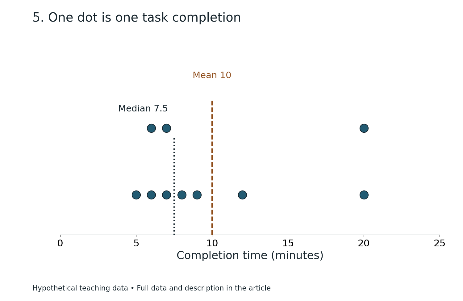
The mean uses every numerical value and is sensitive to extremes. The median marks the middle of an ordered dataset and can describe a typical location when the distribution is strongly skewed. Neither is automatically superior. The choice should follow the question.
Spread matters because similar centres can conceal very different experiences. Two services can have the same average waiting time while one delivers fairly consistent waits and the other combines many short waits with a few very long ones. The second service may need a different operational response.
Start with an appropriate plot and check the actual observations where feasible. Label units, explain the scale and avoid graphical choices that exaggerate or flatten differences. Categories should mean what their labels suggest. If a chart excludes part of the population or period, state that visibly.
For a learner, compare mean, median, minimum and maximum, then explain what each adds. The exercise is complete when the description says something useful about the underlying situation, not simply when four calculations have been performed.
A summary is a choice about what to preserve. Responsible statistics makes that choice explicit.
This invented example uses five waiting times: 2, 3, 4, 5 and 36 minutes. Their sum is 50 minutes, so the mean is 10 minutes. The median is 4 minutes because 4 is the middle value in the ordered list.
Both calculations are correct. “The average wait was 10 minutes” may nevertheless leave readers with a poor picture of the experience. Four people waited five minutes or less, while one person waited 36 minutes. That long wait deserves explanation rather than being hidden inside the mean.
Do not automatically delete 36 as an outlier. Check whether it is a recording error, a different service type or a real difficult case. If it is valid, removing it changes the question and may conceal the people most affected by a service problem.
A better report gives the centre and the distribution. It might state the five observations for this tiny illustration, distinguish the median from the mean and investigate the long wait. With a larger operational dataset, suitable percentiles and subgroup analysis could add useful detail.
The decision depends on purpose. Staffing for total workload may require one view; understanding a typical person’s wait may require another; protecting people from excessive waits may require particular attention to the upper tail.
The gold standard is not to choose whichever average makes performance look best. It is to explain the experience well enough to guide the next action.
A count tells us how many events occurred. A rate or proportion relates a count to an appropriate denominator. Confusing these quantities can reverse the apparent meaning of a comparison.
Suppose one branch records 20 complaints and another records 10. The first branch may appear worse until we learn that it handled 2,000 visits while the second handled 200. The simple complaint proportions are 1% and 5%, respectively. That does not settle every quality question, but it changes the initial interpretation.
Now check comparability. Were complaints recorded using the same definition? Did customers have equal opportunities to report? Were the visits similar in complexity? Did the branches serve different populations? A denominator repairs one problem while leaving other possible differences.
Time also belongs in the explanation. Daily events, monthly totals and annual rates should not be compared as though their exposure periods were identical. A changing denominator can produce an apparent trend even when the underlying event process is more stable.
Students should practise writing the numerator and denominator in words before entering numbers. “Successful applications divided by complete eligible applications reviewed during the period” is more informative than a bare percentage.
The final report should preserve that definition. A percentage without a denominator is an invitation to guess, and a fair comparison should not require the reader to reconstruct its basic meaning.
Imagine two groups in a teaching illustration. In the first, 40 out of 100 students complete a task. In the second, 50 out of 100 complete it. The completion proportions are 40% and 50%.
The absolute difference is 10 percentage points. The relative increase compared with the first group’s proportion is 10 divided by 40, or 25%. Saying “completion improved by 25%” without the original proportions can make the change sound different from what a reader imagines.
Neither form is inherently wrong. They answer different questions. The absolute difference describes the change in proportion on the original scale. The relative increase describes the change compared with the baseline. A clear explanation can give both.
The comparison still does not establish why the groups differ. Were students assigned randomly? Did the task, support, timing and measurement match? Were the groups comparable before the intervention? Was completion the outcome specified in advance?
This is where arithmetic ends and study design becomes essential. A correct percentage cannot manufacture a causal conclusion from an unsuitable comparison.
A useful reporting sentence for this example is: “Completion was 50% in the second group and 40% in the first, a difference of 10 percentage points; the design and uncertainty must be examined before attributing that difference to the programme.” That sentence keeps the result and its boundary together.
| Measure | Group 1 | Group 2 |
|---|---|---|
| Task completions | 40 of 100 | 50 of 100 |
| Completion proportion | 40% | 50% |
| Absolute difference | Compared with Group 1 | 10 percentage points |
| Relative increase | Compared with Group 1 | 25% |
Association means variables vary together in the observed data. Causation concerns what changes when an intervention or condition changes. The first can provide clues about the second, but the two are not interchangeable.
A confounding factor can influence both the exposure and outcome under study. Students who choose an optional workshop may already differ in motivation, available time or prior understanding. Comparing their later performance with non-attendees may mix the workshop’s contribution with those differences.
Random assignment can help create comparable groups in expectation when implemented appropriately. It is not a guarantee that every small sample will be perfectly balanced, and it does not repair every later problem. Non-compliance, missing outcomes, measurement changes and departures from the intended analysis can still matter.
Observational studies can be valuable and sometimes essential. Their conclusions require methods and assumptions suited to the situation. Statistical adjustment does not automatically remove every unmeasured difference or prove causation.
Ask what alternative explanation the study design rules out and what it leaves open. This is a better habit than treating one label, such as “experiment” or “large dataset,” as a complete quality judgement.
For a classroom investigation, identify the intended change, the outcome and the variables that could influence both. A strong explanation says why the chosen comparison is informative and what uncertainty remains.
Different samples from the same population can produce different estimates. Sampling uncertainty describes part of that variation. It is distinct from measurement error, missing-data bias and model misspecification, although these can interact in practice.
An interval estimate communicates a range according to a specified method and set of assumptions. It should be interpreted in that framework. A frequentist confidence interval is not automatically a statement that the fixed unknown parameter has a particular probability of lying inside the one realised interval.
For beginners, the practical lesson is simpler: an estimate needs context about precision, method and assumptions. A narrow interval does not remove bias from a poorly selected sample. A wide interval may mean the data are compatible with a range of materially different possibilities.
Avoid turning overlap rules into universal tests. Whether two intervals overlap is not a general substitute for analysing the actual difference using an appropriate method. Likewise, a result described as uncertain is not necessarily useless; it may identify what additional evidence is needed.
When reading an interval, ask what quantity it concerns, which uncertainty it represents and which assumptions support it. When reporting one, explain the result in ordinary language alongside the technical expression.
Statistics becomes more useful when uncertainty is part of the answer rather than a footnote apologising for it.
A p-value is a model-based quantity used in statistical testing. Roughly, it assesses how unusual the observed result or a more extreme result would be under a specified null model and its assumptions. It is not the probability that the hypothesis is true.
The American Statistical Association’s statement on p-values is a primary reference for avoiding common misinterpretations. It emphasises that a threshold alone should not decide a scientific or practical conclusion, and that statistical significance does not measure effect size or importance.
The practical repair is to report the estimated effect, relevant uncertainty, design, assumptions and context. A tiny difference can be statistically detectable in a large dataset yet have little practical value. A potentially important difference in a small study may remain too uncertain for a strong conclusion.
Do not describe a result just above a conventional threshold as proof of no effect. Do not describe a result just below it as complete proof of a useful intervention. Both shortcuts replace reasoning with a label.
For students, separate three questions: what difference was estimated, how uncertain is the estimate, and would that difference matter in this setting? Those questions remain useful even when the formal method is beyond the current syllabus.
The aim is a conclusion proportionate to all the evidence, not a competition to produce the smallest number.
An empty cell can mean several things: not measured, not applicable, refused, lost, below a detection limit or genuinely zero. These meanings should not be collapsed into one convenient replacement value.
Missingness can affect interpretation when the observed cases differ from the missing cases. A follow-up survey that mainly reaches satisfied participants may overstate satisfaction. A sensor that fails during the most severe conditions can underrepresent precisely the events the study needs to understand.
Begin by documenting how many observations are missing, for which variables and at what stage. Compare available information about observed and missing groups where appropriate. Explain exclusions and preserve a record of the rules used.
There is no universally correct repair. Complete-case analysis, weighting, imputation and sensitivity analysis each involve assumptions and may suit different settings. Advanced methods do not make the reason for missingness disappear. Their suitability must be argued.
For a school investigation, an honest small table is often enough to improve the explanation: number assigned, number measured, number missing and known reasons. A student can then state how the gaps limit the conclusion.
The gold standard keeps missing information visible. A smaller transparent dataset can support a more trustworthy conclusion than a polished table that quietly removes inconvenient cases.
Exploratory analysis helps us notice patterns and generate questions. Confirmatory analysis tests a specified question using a planned approach. Both are useful, but they carry different evidential meanings.
If a researcher tries many outcomes, subgroups and transformations, an interesting result may appear through the search process. Reporting only that result as though it were the original single test exaggerates the evidence. The problem is selective presentation rather than curiosity itself.
A better workflow records which questions and methods were specified before seeing the relevant results. Exploratory findings are labelled honestly. Important new patterns can then motivate suitable follow-up using fresh data or an appropriately planned analysis.
Changing a method may be justified when an assumption fails or a recording problem is discovered. The change and its reason should remain visible. A transparent revision is stronger than pretending the analysis never changed.
For students, keep two notebook pages: “planned question” and “new questions noticed.” This simple separation protects a useful discovery from being overstated. A surprising result becomes the beginning of another investigation rather than an excuse to rewrite the original aim.
Statistical integrity does not require knowing every answer in advance. It requires a truthful account of how the answer was reached.
A statistical model represents relationships using assumptions and a mathematical structure. It can help explain patterns or predict new observations. The intended job influences how the model should be evaluated.
A model that fits the existing dataset closely may perform poorly on new cases. It may have captured noise, used information that would not be available at prediction time or benefited from a convenient but unrepresentative sample. Evaluation should match the future use.
Keep training and evaluation processes appropriately separated. For time-dependent data, random splitting may be unsuitable if it lets future information influence a past prediction. For repeated observations from the same people or sites, the split should recognise those relationships.
Overall accuracy can hide failures in particular groups or rare important events. Calibration, false positives, false negatives and the cost of errors may matter more than one headline score. The appropriate measures depend on the decision.
A model’s success also has a domain. Changes in populations, instruments, policy or behaviour can weaken earlier performance. Monitoring and revision become part of responsible use.
For a learner, compare a model with a simple baseline and inspect the cases it gets wrong. Ask whether the errors have a pattern. Understanding failure often teaches more than another decimal place in a score.
Choose a graphic to match the question. A line chart can show ordered change over time. A scatterplot can reveal a relationship between two numerical variables. A histogram can show distribution. A bar chart can compare categories. None is automatically the best chart for every dataset.
Axes should have clear labels and units. A truncated scale may be appropriate in some analytical contexts, but it should not conceal how the display changes the visual impression. Category order, bin width, colour and missing periods can all affect interpretation.
Keep the data’s structure visible. Connecting unrelated categories with a line can suggest a continuity that does not exist. Presenting irregular time intervals at equal spacing can distort a trend. Showing only a final average can hide changes during the period.
A useful caption states what the reader is seeing, the source and any important limitation. If a chart combines estimates from different definitions or methods, explain the comparison rather than leaving it visually seamless.
Accessibility matters too. Use readable labels, sufficient contrast and meaning that does not depend solely on colour. Provide the key numerical values or an appropriate table when readers need exact comparisons.
The gold standard of a graph is not decorative complexity. It is that another person can identify the pattern and understand the conditions under which the pattern is meaningful.
The same statistical habits transfer across settings, but the variables and decisions differ. In school Science, the task may be to compare treatment groups fairly. In a public service, it may be to understand who experiences delays. In engineering, it may be to distinguish routine process variation from a meaningful change.
Context determines what counts as a useful difference. A small change can matter greatly when repeated across many cases, while a larger change may have little value if the measurement is unrelated to the intended outcome. Costs, benefits and consequences belong beside numerical evidence.
Subgroups also matter. An overall improvement can coexist with a worsening experience for a smaller group. Before declaring success, examine whether the summary hides important differences, while avoiding unsupported conclusions from tiny subgroup samples.
Good statistical work therefore requires conversation with people who understand the setting. A statistician may identify the analytical issue; a domain expert may explain why the recording process changed or why two categories should not be combined.
For learners, start with a familiar decision and ask what data would actually improve it. This develops a stronger foundation than collecting numbers because a chart is required.
The subject becomes practical when the analysis leads to a justified action, a narrower claim or a better question for the next investigation.
If calculations are difficult, begin with the quantity and units. Write the formula in words, substitute labelled values and check whether the answer has the expected scale. Estimation can reveal a misplaced decimal before a calculator produces a polished error.
If interpretation is difficult, return to the data-generating process. Who was measured, how and when? Separate the recorded pattern from the proposed explanation. Many interpretation mistakes come from skipping this stage rather than from weak arithmetic.
If comparisons are difficult, write the group definitions, denominators and observation periods side by side. Check whether the measurements mean the same thing. A comparison that fails these checks may need redesign before any formal test.
If uncertainty is difficult, practise describing several plausible values rather than reaching immediately for a binary verdict. Ask how the decision would change across that range. This makes the practical meaning of precision easier to understand.
If written answers are vague, use a four-sentence structure: identify the result, connect it to the question, explain the relevant design or mechanism and state the main limitation. Add detail when it changes the judgement.
The next learning step should match the actual bottleneck. More exercises on averages will not repair confusion about causal inference, and advanced testing will not repair unclear denominators.
A website reports that 90% of respondents enjoyed a new event. What should you ask first? Identify who could respond, how many people responded, the wording of the question and whether non-attendees or dissatisfied participants were less likely to reply. The percentage describes the observed respondents before it describes any wider population.
A factory’s average output rose after new equipment arrived. Does the machine necessarily explain the change? No. Staffing, demand, product mix, operating hours, measurement rules and other changes may contribute. The comparison needs a design and context capable of supporting the intended causal claim.
A survey doubles its sample size. Does every uncertainty halve? No. Sampling precision depends on the method and design, and several sources of bias may remain unchanged. Larger samples do not automatically correct coverage or measurement problems.
A dataset contains an unusually high valid value. Should it be removed? Investigate its meaning. If it belongs to the target population, deleting it may hide an important part of the phenomenon. Report justified exclusions and consider suitable summaries.
An analysis finds no statistically significant difference. Has it proved equivalence? Not automatically. The estimate, uncertainty, design and any formal equivalence framework matter. An inconclusive comparison can remain compatible with meaningful differences.
In each answer, the numerical technique is only one part of the reasoning. The stronger habit is to identify what information would change the conclusion.
Is Statistics the same as Mathematics? It uses mathematics, but its practical work also involves study design, measurement, context and reasoning from incomplete observations. A correct derivation does not by itself establish that a model suits the data.
Is a larger sample always better? A larger suitable sample can improve precision for some questions. It does not automatically repair biased selection, unclear definitions or unsuitable measurements.
Which average should I use? Choose according to the question and distribution. Explain the choice and include spread or other features when one centre would hide important variation.
Can correlation ever be useful? Yes. It can describe patterns, support prediction and generate hypotheses. It should not be promoted automatically into a causal conclusion.
Does statistical significance mean importance? No. Effect size, uncertainty and practical context are separate considerations.
Can artificial intelligence perform the analysis? Tools can help organise data, generate code and propose methods. The user still needs to verify definitions, assumptions, calculations, privacy and interpretation. A confident generated explanation can contain errors.
What is the first step towards better statistical thinking? Before calculating, describe the question, population, unit of observation and measurement process. That short description prevents many later mistakes.
What should a good final report contain? Enough information to understand what was studied, how the evidence was obtained, what was estimated and what limits the conclusion. The reader should be able to see why the claimed result follows.
Chapter 20 of 21
20. Specialist articles across the eduKate ecosystem
For a worked reconstruction with explicit bounds on rounded group means, continue to Rounded Group Means and False Precision in a Combined Variance.
These published companion articles develop the branches introduced in this guide. Choose the group that matches your question; the directory connects related subjects without treating their distinct professional requirements as interchangeable.
Learn the foundations
- The Gold Standard of Teaching Statistics | Questions, Variation and Valid Inference
- The Gold Standard of a Ministry of Education | National School Census, EMIS and Education Statistics Data Quality
- The Gold Standard Of Science
Design and interpret investigations
- The Gold Standard Of School Scientific Exploratory Findings Confirmation Planning
- The Gold Standard Of School Scientific Pre-Specified Outcome Definitions
- The Gold Standard of Cross-Language Interview Research Services | Faithful Questions and Context-Rich Evidence
- The Gold Standard of Multilingual Focus Group Research Services | Fair Participation and Comparable Insights
- The Gold Standard of Cross-Language Survey Research Services | Comparable Questions and Trustworthy Responses
- The Gold Standard Of School Scientific Detection Bias In Observations
- The Gold Standard Of School Scientific Replication Disagreement Interpretation
- The Gold Standard Of School Scientific Baseline Balance Assessment
- The Gold Standard Of School Scientific Missing Outcome Data Analysis
- The Gold Standard Of School Scientific Random Assignment To Treatment Groups
- The Gold Standard Of School Scientific Control Group Design
- The Gold Standard Of School Scientific Negative Findings Interpretation
- The Gold Standard Of School Scientific Presentation Question Handling
Practise with concrete cases
- The Gold Standard of Industrial Temperature Sensor Calibration Services | Traceable Readings, Honest Uncertainty and Reliable Processes
- The Gold Standard Of Urban Environmental API Temporal Aggregation Unit Consistency
- Gold Standard Practical Case Study 191 | The Student Confidence Survey Reported 4.1 Out of 5 but One Question Was Scored Backwards
- Gold Standard Practical Case Study 190 | The Botanical Survey Counted Forty Plant Names as Forty Species but Thirteen Were Synonyms
- Gold Standard Practical Case Study 185 | The Water Survey Averaged pH 6 and pH 8 and Reported Neutral Water
- Gold Standard Practical Case Study 138 | The Neighbourhood Survey Collected 150 Replies but Heard from Only 100 Households
Use these primary references to follow the named frameworks and scientific resources. The worked cases and practical teaching explanations in this article are original illustrations; formal applications require the sources and requirements relevant to the particular setting.
- NIST/SEMATECH — e-Handbook of Statistical Methods
- NIST — measurement-process characterisation
- American Statistical Association — statement on statistical significance and p-values
Contents · Previous chapter · The Gold Standard master guide