
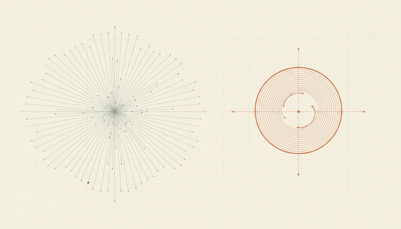
A flow can preserve the area of a moving patch while stretching some of its lines and shortening others. Zero divergence controls a local area or volume balance. It does not say that the moving material keeps every length, angle or shape.
The short answer is to distinguish the determinant from the full deformation. A smooth flow with zero divergence along its trajectories preserves material area in two dimensions, starting from the identity map. Length preservation requires the stronger condition that the deformation’s matrix preserves dot products. An area-preserving shear provides a concrete counterexample.
This original mathematical lesson continues Vector Calculus, Learning That Transfers into Life and How X Works. Coordinates are Cartesian and dimensionless unless units are stated. The examples describe ideal maps and velocity fields; they are not complete physical models of a particular fluid or material.
eduKateSG · Vector Calculus
Find your next learning step
Track labelled material lines while checking area and shape separately.
ROUTE 1 · CHAPTERS 1–7
Follow a moving patch
Separate particle labels, velocity and the exact shear map.
ROUTE 2 · CHAPTERS 8–15
Measure directional change
Check dot products, extreme stretches and evolving direction.
ROUTE 3 · CHAPTERS 16–23
Connect operators to history
Compare rotation, extension, material area and final-state evidence.
ROUTE 4 · CHAPTERS 24–30
Challenge approximations and bounds
Test numerical steps, finite strain and hidden deformation.
ROUTE 5 · CHAPTERS 31–35
Audit and practise
Build a usable evidence record and transfer the distinctions.
Chapter contents
Follow a moving patch · Chapters 1–7
1. Start with a patch rather than one arrow
2. Keep position, velocity and displacement distinct
3. Define a shear velocity field
4. Calculate divergence and curl without conflating them
5. Map the square's four corners
Measure directional change · Chapters 8–15
8. Derive the length change for an arbitrary direction
9. Use the dot-product test for full length preservation
10. Find the largest and smallest stretch at unit shear
11. Keep initial and final principal directions separate
12. Generalise the extreme stretch formula
13. Distinguish instantaneous rate from accumulated stretch
14. Derive the instantaneous length rule directly
15. Follow one rotating material direction through the rate formula
Connect operators to history · Chapters 16–23
16. Compare a rotation with the same curl
17. Show that zero curl does not prevent stretching either
18. Connect divergence to the area Jacobian
19. Change the time history and test the condition
20. Distinguish a material patch from a fixed control region
21. Keep the two-dimensional and three-dimensional statements aligned
Challenge approximations and bounds · Chapters 24–30
24. Test a numerical update rather than trusting its label
25. Compare two independent checks on an approximation
26. Work a changed shear without using the old diagram
27. Do not use an infinitesimal strain identity as a finite one
28. Turn a shear-history bound into a stretch bound
29. Test how much the two operator readings leave unidentified
30. Keep local stretch separate from a curved line's total length
Audit and practise · Chapters 31–35
31. Build an evidence record for a material-motion claim
32. Repair and extend the learning route
33. Questions readers often ask
CHAPTER 1 OF 35 · Follow a moving patch
1. Start with a patch rather than one arrow
Imagine a unit square marked by four identifiable material particles. Move the top edge to the right while leaving the bottom edge in place, with a displacement proportional to height. The square becomes a parallelogram.
Its base and perpendicular height can both remain one, so its area remains one. Yet the sloping sides are longer than the original vertical sides, and its right angles have changed. This picture already separates area preservation from rigid motion.
A velocity arrow at one location cannot show the whole distinction. Shape change depends on differences between the motion of neighbouring particles. Begin by naming which particles form the patch and following those same identities. Replacing them with whichever particles happen to occupy a fixed square later would ask a different question about a fixed region of space.
CHAPTER 2 OF 35 · Follow a moving patch
2. Keep position, velocity and displacement distinct
Let (X,Y) label a particle’s initial position. Its later position is (x(X,Y,t), y(X,Y,t)). The mapping from initial labels to current position is the flow map.
Velocity gives the time derivative of current position while following that particle. Displacement is current position minus initial position. A spatial gradient of velocity and a gradient of the flow map are therefore different objects, even though both can be written as matrices.
For a steady velocity field, the arrows at fixed locations do not change with time. Material particles can nevertheless continue to move through those arrows and accumulate deformation. Steady does not mean stationary particles or unchanged material shape. Keep the particle labels in the notation until that distinction is secure; otherwise a time-independent formula can be mistaken for a claim that nothing continues to happen.
Use v(x,y) = (s y, 0), with constant shear rate s. If positions are measured in metres and time in seconds, s has units per second so that s y has velocity units.
The y-velocity is zero, so a particle keeps its initial Y coordinate. Its x-velocity is consequently sY, constant along its trajectory. Integrating from time zero gives x = X + stY and y = Y.
Define accumulated shear γ = st. The flow map is (X,Y) ↦ (X + γY,Y). This is an exact solution of the stipulated velocity field, not a first-order approximation in time. Negative s shears in the opposite direction. The field can be studied mathematically on the whole plane, while a real experiment would require boundaries and forces that this kinematic example does not specify.
CHAPTER 4 OF 35 · Follow a moving patch
4. Calculate divergence and curl without conflating them
For the shear field, divergence is ∂(sy)/∂x + ∂0/∂y = 0. The planar scalar curl is ∂0/∂x − ∂(sy)/∂y = −s.
Zero divergence therefore coexists with nonzero local rotation information. Neither calculation yet gives the length of a material line after a finite time. That requires following the flow map.
The sign of curl depends on the declared right-handed coordinate convention. With positive x to the right and positive y upward, positive s makes higher particles move faster to the right and gives negative scalar curl. Changing the viewing convention without changing the algebra can create an apparent sign disagreement. The useful habit is to identify the operator’s question first: divergence concerns outward balance, curl concerns local circulation, and finite deformation concerns how labelled separations evolve.
Take γ = 1. The initial corners (0,0), (1,0), (1,1) and (0,1) become (0,0), (1,0), (2,1) and (1,1).
The transformed bottom side has vector (1,0), while the transformed left side has vector (1,1). Their parallelogram area is the absolute determinant 1 × 1 − 0 × 1 = 1. Their lengths are one and √2.
The perimeter has increased from four to 2 + 2√2, approximately 4.828. The angle between these two sides is 45 degrees rather than 90. Area, perimeter and angle have changed in different ways. Counting the same four particles or preserving their enclosed area does not imply that every geometric quantity associated with them is preserved. This small coordinate calculation is an independent check on the original sketch.
The derivative of the flow map with respect to initial coordinates is F = [[1,γ],[0,1]]. A small initial separation dX becomes dx = F dX. For this affine map, the same relationship is exact for any separation, not merely an infinitesimal one.
Its determinant is one for every γ. That gives the area ratio for the map. For a three-dimensional extension that leaves z unchanged, the corresponding three-by-three determinant is also one and volume is preserved.
The determinant compresses much of the matrix’s information into one scalar. Matrices with the same determinant can have different effects on lengths and directions. This is why a volume-balance check is necessary for the stated conservation property but insufficient for a rigid-motion claim. The next calculation retains the full matrix instead of replacing it by its determinant.
At γ = 1, a unit horizontal vector (1,0) becomes (1,0) and keeps length one. A unit vertical vector (0,1) becomes (1,1) and has length √2.
A third initial unit vector is (1,−1)/√2. It becomes (0,−1)/√2 and has length 1/√2. Thus one direction is unchanged, another lengthens, and another shortens under exactly the same area-preserving map.
These are labelled material directions, not three different flows. The comparison refutes the claim that area preservation forces all lines to stay unchanged. It also shows why testing only the horizontal direction would be inadequate. A favourable single direction can conceal a transformation’s effect elsewhere. Choose deliberately different directions when checking a geometric claim about every possible material line.
CHAPTER 8 OF 35 · Measure directional change
8. Derive the length change for an arbitrary direction
Let an initial unit vector be n = (cos θ, sin θ). The transformed vector is (cos θ + γ sin θ, sin θ). Its squared length is 1 + γ sin(2θ) + γ² sin²θ.
This formula includes the three checks above. At θ = 0 the ratio is one. At θ = π/2 it is 1 + γ². At θ = −π/4 with γ = 1 it is one half.
The cross term is essential. Adding the squared effects of the two original coordinate directions without it would miss the interaction between the horizontal and vertical components after shearing. Length is calculated after the vector components are combined. This is another reason that a scalar balance such as divergence cannot replace the directional information in the complete transformation.
CHAPTER 9 OF 35 · Measure directional change
9. Use the dot-product test for full length preservation
For a matrix F, the squared transformed length is nᵀFᵀFn. Every vector keeps its length precisely when FᵀF = I in these Euclidean coordinates.
For the shear, FᵀF = [[1,γ],[γ,1 + γ²]]. This equals I only when γ = 0. Its determinant is still one, because det(FᵀF) = det(F)².
An orthogonal matrix preserves dot products, lengths and angles. An area-preserving matrix need only have determinant of absolute value one. Our flow map has positive determinant one, consistent with continuous orientation-preserving evolution from the identity. The stronger orthogonality condition is exactly what the nonzero shear fails. Naming the two tests makes it possible to explain the missing implication rather than simply memorise a counterexample.
CHAPTER 10 OF 35 · Measure directional change
10. Find the largest and smallest stretch at unit shear
At γ = 1, the symmetric matrix FᵀF is [[1,1],[1,2]]. Its characteristic equation is λ² − 3λ + 1 = 0, giving eigenvalues (3 ± √5)/2.
The extreme length ratios are the square roots: σ_max = (1 + √5)/2, approximately 1.618, and σ_min = (√5 − 1)/2, approximately 0.618. These are the singular values of F.
Their product is one, in agreement with area preservation. Neither has to equal one individually. The expanding direction and contracting direction compensate in their area product, rather than forcing every individual direction to remain fixed. Computing these extremes gives a complete directional length check for the affine map, beyond the three selected vectors used earlier.
CHAPTER 11 OF 35 · Measure directional change
11. Keep initial and final principal directions separate
Let φ = (1 + √5)/2. An initial vector proportional to (1,φ) is an eigenvector of FᵀF for the largest squared stretch. Its initial angle is about 58.28 degrees above the x-axis.
After unit shear, it becomes proportional to (1 + φ,φ), whose angle is about 31.72 degrees. The direction giving the largest initial-to-final stretch is therefore not pointing along the same line before and after the deformation.
Eigenvectors of FᵀF describe initial directions; eigenvectors of FFᵀ describe final principal directions. Confusing those spaces can produce a plausible but misplaced arrow on a diagram. A learner should label which configuration contains each direction. The singular value connects the two lengths, while the full matrix connects the vectors themselves.
CHAPTER 12 OF 35 · Measure directional change
12. Generalise the extreme stretch formula
For arbitrary real γ, the extreme singular values are (√(γ² + 4) + |γ|)/2 and (√(γ² + 4) − |γ|)/2. Their product remains one.
The absolute value reflects the fact that reversing shear changes the directional arrangement but not the pair of extreme stretch magnitudes. At γ = 0 both values are one. As |γ| becomes large, the maximum grows approximately like |γ|, while the minimum decreases approximately like 1/|γ|.
Area preservation therefore places no finite upper bound on the largest stretch if accumulated shear is unrestricted. A bound on determinant alone is not a bound on distortion. To bound how long a material line can become, one needs additional information about the velocity gradients, elapsed history or the transformation itself. That limitation matters whenever a conservation check is being used as a substitute for a deformation check.
CHAPTER 13 OF 35 · Measure directional change
13. Distinguish instantaneous rate from accumulated stretch
The velocity-gradient matrix for v = (sy,0) is L = [[0,s],[0,0]]. Split it into its symmetric part D = (L + Lᵀ)/2 and antisymmetric part W = (L − Lᵀ)/2.
Here D = [[0,s/2],[s/2,0]] and W = [[0,s/2],[−s/2,0]]. For a current unit material direction m, the instantaneous fractional length-change rate is mᵀDm.
The antisymmetric part contributes zero to mᵀWm. It influences direction, which in turn changes how the material line encounters D later. It is therefore wrong to infer that W can simply be discarded from a finite deformation calculation. The instantaneous stretch formula and the accumulated map answer different time questions, connected by the changing material direction.
CHAPTER 14 OF 35 · Measure directional change
14. Derive the instantaneous length rule directly
Let a current small material separation be a(t), evolving according to ȧ = L a. Differentiate its squared length: d(aᵀa)/dt = aᵀ(Lᵀ + L)a = 2aᵀDa.
Writing a = ℓm with unit m gives 2ℓℓ̇ = 2ℓ²mᵀDm, so ℓ̇/ℓ = mᵀDm. This derivation explains why the symmetric part controls instantaneous length change.
For unit directions at plus and minus 45 degrees in the positive-s shear, the initial fractional rates are plus s/2 and minus s/2. But those directions generally turn as the shear proceeds. Exponentiating those initial rates as though the same material directions remained principal forever would answer another problem. The exact finite-time singular values already show the result that the full trajectory calculation must recover.
CHAPTER 15 OF 35 · Measure directional change
15. Follow one rotating material direction through the rate formula
An initially vertical unit line in the constant-s shear becomes a(t) = (st,1). Its length is ℓ(t) = √(1 + s²t²), and its current unit direction is m(t) = (st,1)/√(1 + s²t²).
Substituting that current direction into D gives mᵀDm = s²t/(1 + s²t²). Directly differentiating ln ℓ produces exactly the same expression. Integrating from zero to T gives ln ℓ(T) = one half ln(1 + s²T²), recovering the finite length formula independently.
At time zero the instantaneous stretch rate of this vertical line is zero. It nevertheless lengthens later because its orientation changes. Treating the initial rate as a constant would predict length one forever and fail this direct check. This calculation shows how a local rate becomes an accumulated change only when it is evaluated along the actual evolving direction. The line’s identity stays fixed while its orientation supplies changing input to the rate equation.
CHAPTER 16 OF 35 · Connect operators to history
16. Compare a rotation with the same curl
Consider the rigid-rotation velocity v_R = (sy/2, −sx/2). Its divergence is zero and its scalar curl is −s, exactly matching the shear’s curl.
Its velocity gradient is entirely antisymmetric, so D_R = 0. The exact flow map is a rotation through angle −st/2. Every material length and angle remains unchanged, and its determinant is one.
The shear and rotation therefore have the same divergence and curl while producing different material stretching. This does not contradict field reconstruction theorems, which require additional domain and boundary information. It demonstrates a local interpretive limit: two scalar operator summaries in a planar comparison do not by themselves provide the full strain-rate information or finite flow map. A curl value cannot be read as the amount of total material deformation.
CHAPTER 17 OF 35 · Connect operators to history
17. Show that zero curl does not prevent stretching either
Now use v_E = (ax, −ay), with constant a. Its divergence is a − a = 0, and its scalar curl is zero. The particle equations integrate to x = eᵃᵗX and y = e⁻ᵃᵗY.
The flow matrix is diagonal with entries eᵃᵗ and e⁻ᵃᵗ. Their product is one, so area remains unchanged. Horizontal lines stretch by eᵃᵗ while vertical lines contract by its reciprocal.
For at = ln 2, the ratios are two and one half. Thus even zero divergence together with zero curl does not force rigid motion. The symmetric gradient can still contain equal-and-opposite extension rates. The field is the gradient of a(x² − y²)/2, showing that having a scalar potential does not imply that neighbouring material particles retain their separation.
CHAPTER 18 OF 35 · Connect operators to history
18. Connect divergence to the area Jacobian
For a smooth flow map, let F be its spatial derivative with respect to initial labels, and J = det F. Along a trajectory, Ḟ = L F, with L the velocity gradient evaluated at the moving particle.
Jacobi’s determinant identity gives J̇ = J trace(L) = J div v. Starting with J(0) = 1, integration gives J(t) = exp(∫₀ᵗ div v(x(τ),τ) dτ), while the flow remains smooth and invertible on the relevant domain.
If divergence vanishes throughout that history, J remains one. This is the precise connection behind material area preservation in two dimensions and volume preservation in three. It is a time-integrated statement along trajectories. Evaluating divergence at one convenient point or at one instant does not establish that the integral vanishes for every material particle being discussed.
CHAPTER 19 OF 35 · Connect operators to history
19. Change the time history and test the condition
Use v(x,y,t) = (t x,0), with dimensionless time. At t = 0, divergence is zero everywhere. Later it equals t.
The exact flow is x = exp(t²/2)X and y = Y. Its area ratio is exp(t²/2), greater than one for positive time. An initial zero-divergence reading has not preserved later area because the condition did not continue to hold.
The determinant formula verifies the result: integrating divergence from zero to t gives t²/2. This changed example tests whether the learner retained the history requirement rather than only the phrase zero divergence. A field observation should always include its spatial and temporal scope. A calculation valid over an entire trajectory cannot be justified by a snapshot whose future conditions are unknown.
CHAPTER 20 OF 35 · Connect operators to history
20. Distinguish a material patch from a fixed control region
A material patch consists of the same labelled particles as they move. A fixed region of space keeps its boundary in place while different particles may enter and leave.
For zero-divergence flow, the net outward volume flux through a suitable closed boundary is zero at a given instant, under the divergence theorem’s conditions. That does not say that no fluid crosses any part of the boundary. Equal entering and leaving contributions can cancel.
Similarly, preserving a moving patch’s area does not mean it remains inside its original square. In our shear, upper corners move to the right even though area stays one. When interpreting a diagram or experiment, ask which boundary is being followed. A fixed observation window and a moving collection of particles can produce different records without disagreeing about the underlying velocity field.
CHAPTER 21 OF 35 · Connect operators to history
21. Keep the two-dimensional and three-dimensional statements aligned
Our planar determinant measures area. Embedding the shear as (x,y,z) = (X + γY,Y,Z) gives determinant one and preserves three-dimensional volume.
It does not preserve every embedded surface area. A unit rectangle spanned by the initial vertical direction and the unchanged z-direction has area one. After unit shear its spanning vectors are (1,1,0) and (0,0,1), whose cross-product magnitude is √2.
Thus a volume-preserving three-dimensional map can change a surface’s area just as an area-preserving planar map can change a line’s length. Each geometric quantity has its own transformation rule. The determinant answers the full-dimensional volume question; lower-dimensional measures depend on orientation and the action of the full map. Keep the dimension of the conserved quantity visible in the statement.
CHAPTER 22 OF 35 · Connect operators to history
22. Use an inverse to check the map
The inverse shear is F⁻¹ = [[1,−γ],[0,1]]. Applying it after F returns every labelled position and separation to its starting value. Its determinant is also one.
At γ = 1, the initially vertical unit vector becomes (1,1). Applying the inverse returns (0,1). This confirms that the earlier length change is reversible as a mathematical mapping, rather than evidence that particles have been created or removed.
Reversibility here is kinematic. It does not establish physical reversibility of a real flow, whose energy dissipation, diffusion or material response would require additional equations. An exact inverse for a coordinate map is a statement about geometric reconstruction. Keeping that scope prevents a correct matrix identity from being turned into a broader physical claim it has not proved.
CHAPTER 23 OF 35 · Connect operators to history
23. Do not infer the whole past from a final identity map
A time-dependent shear with rate s(t) has accumulated shear γ(t) = ∫₀ᵗ s(τ)dτ. If positive and negative contributions cancel, the final map can be the identity.
For example, use rate one for one time unit and minus one for the next. At the midpoint γ = 1 and the square is distorted as before. At the end γ = 0 and the ideal map returns it to its original shape.
A final unchanged shape therefore does not prove that every intermediate length was unchanged. This matters when the question concerns peak stretch rather than final stretch. Within our example the maximum singular value at the midpoint is about 1.618, even though its final value is one. Preserve the time quantity being assessed: final configuration, instantaneous rate and maximum over a history are different outputs.
CHAPTER 24 OF 35 · Challenge approximations and bounds
24. Test a numerical update rather than trusting its label
An exact divergence-free flow need not remain area-preserving after a numerical approximation. Consider the extension field v = (ax,−ay). One forward Euler step of size h maps positions by diag(1 + ah, 1 − ah).
The step determinant is 1 − a²h², rather than one. With ah = 1/2, it equals three quarters, although the exact map over the same step preserves area.
The velocity field’s zero divergence is not the source of the discrepancy. The finite-step approximation has introduced an area error. A numerical test should therefore examine the computed map and its convergence, not merely verify the analytic divergence formula. This is a useful example of distinguishing a mathematical model from the algorithm used to approximate its trajectories.
CHAPTER 25 OF 35 · Challenge approximations and bounds
25. Compare two independent checks on an approximation
For the rigid rotation with angular speed ω, a forward Euler step has matrix [[1,−ωh],[ωh,1]]. Its determinant is 1 + ω²h², so it expands area and lengths, although the exact rotation preserves both.
For n steps across fixed duration T, its area factor is (1 + ω²T²/n²)ⁿ. This approaches one as n grows, but exceeds one for every finite n when ωT is nonzero.
Checking both area and length reveals the approximation’s behaviour more clearly than checking a plotted trajectory alone. A coarse spiral may be a numerical artefact rather than a property of the stipulated field. Compare against an exact solution where available, refine the step and keep numerical error separate from an inference about the real system. One successful invariant check does not establish every other geometric property.
CHAPTER 26 OF 35 · Challenge approximations and bounds
26. Work a changed shear without using the old diagram
Set γ = 2. An initially vertical unit vector becomes (2,1), with length √5. The unit horizontal vector remains unchanged. Area remains one.
The extreme stretch ratios are √2 + 1 and √2 − 1, approximately 2.414 and 0.414. Their product is one. For initial direction (1,−1)/√2, the transformed vector is (−1,−1)/√2, whose length happens to remain one in this changed case.
That last result differs from its contraction at unit shear. A particular direction can shorten at one accumulated shear and regain its original length later, even as the largest possible stretch continues to grow. The learner should calculate from the specified map rather than classify a direction permanently as expanding or contracting from one earlier example.
CHAPTER 27 OF 35 · Challenge approximations and bounds
27. Do not use an infinitesimal strain identity as a finite one
For the unit shear, the displacement is (Y,0). Its gradient has zero trace. The symmetric infinitesimal strain matrix is [[0,1/2],[1/2,0]], also with zero trace. These are useful small-deformation descriptors, but the actual finite length changes require FᵀF.
The Green strain E = (FᵀF − I)/2 is [[0,1/2],[1/2,1/2]], whose trace is one half. This does not contradict determinant one. Trace of a strain approximation and exact volume ratio are different quantities once finite terms matter.
In this example the γ² term is the missing finite contribution. Dropping it would predict the wrong squared length for an initially vertical line. A good approximation states which terms it neglects and over what range the omission is acceptable. Saying that a strain matrix has trace zero is not an exact proof about every finite geometric measure associated with the motion.
CHAPTER 28 OF 35 · Challenge approximations and bounds
28. Turn a shear-history bound into a stretch bound
Suppose the rate history is known only to satisfy ∫₀ᵀ |s(t)|dt ≤ G. Then the accumulated shear obeys |γ(T)| ≤ G. Since the largest singular value increases with |γ|, its upper bound is (√(G² + 4) + G)/2.
For G = 1 this is about 1.618. This is a bound on the largest final stretch within this particular family of shear maps. It is more informative than determinant one because it uses an additional limit on accumulated shear.
Sign changes may make the actual final γ much smaller than G. If the question concerns the largest stretch at any intermediate time, the same total-absolute-rate bound controls every partial integral, but an endpoint value γ(T) alone does not. Distinguish a bound on the whole history from a measurement of its final net result. The conditions determine which stretch question the number can answer.
CHAPTER 29 OF 35 · Challenge approximations and bounds
29. Test how much the two operator readings leave unidentified
Consider the family v_a = (sy + ax, −ay), where a is any constant. Every member has divergence zero and scalar curl −s. Yet its symmetric velocity gradient is [[a,s/2],[s/2,−a]].
The extreme instantaneous fractional stretch rates are plus and minus √(a² + s²/4). Their magnitude can be arbitrarily large as |a| increases, while the divergence and curl remain exactly the same. Thus those two readings alone cannot even bound the largest instantaneous stretching rate in this family.
This is a direct identification test: construct several fields agreeing on the supplied information and compare the desired output. If the output differs, additional evidence is needed. Boundary conditions, more velocity measurements or a justified field model could restrict a. A colourful arrow plot does not add that missing information unless its arrows actually represent observations or a specified model.
CHAPTER 30 OF 35 · Challenge approximations and bounds
30. Keep local stretch separate from a curved line's total length
For a nonlinear changed case, use the map x = X + Y² and y = Y. Its Jacobian determinant is one everywhere, but a vertical segment from (0,0) to (0,1) becomes a parabola rather than a straight side.
The end-to-end chord has length √2. The curve’s actual length is ∫₀¹ √(1 + 4Y²)dY = √5/2 + asinh(2)/4, approximately 1.479. These are different quantities. Its local vertical-direction stretch varies from one at Y = 0 to √5 at Y = 1.
The affine shear allowed one matrix to transform an entire finite segment exactly. For a nonlinear map, its derivative describes local separations, and the total length of a mapped curve requires accumulating the local contribution along that curve. Replacing the curve by the straight line between its transformed endpoints discards its bending. The area-preservation conclusion remains valid while the length calculation becomes more spatially detailed.
CHAPTER 31 OF 35 · Audit and practise
31. Build an evidence record for a material-motion claim
A useful record identifies the velocity field, coordinate conventions, time interval, initial labels and domain. It states whether the flow map is exact, inferred from data or numerically approximated.
For a conservation claim, record the relevant divergence history and determinant. For a length claim, record the material direction or the extreme singular values. For a rotation claim, check dot products or the symmetric rate tensor rather than using curl alone.
If working with measurements, spatial resolution and gradient estimation introduce further uncertainty. A few arrows or one trajectory do not determine every neighbouring velocity difference. Explain which observations support the proposed map and which features remain model assumptions. The goal is a statement another reader can test, such as this labelled line’s length ratio over this interval, rather than an unqualified claim that the flow does not deform.
If area and length are being confused, return to the sheared unit square and calculate its determinant and side lengths separately. If velocity and displacement are mixed, solve one particle’s differential equation before introducing matrix notation.
For stabilisation, compare shear, rigid rotation and equal-and-opposite extension without supplying their labels. Ask which preserve area, which preserve all lengths, and which have zero curl. Require one independent calculation for each classification.
For extension, let the shear rate change with time, investigate an initial material line with a general angle, or compare an exact map with an Euler approximation. Each task changes one condition while retaining the same labelled-particle question. A dependable answer identifies the changed relationship and its limits, rather than adding more operator formulas without deciding what they measure.
Does incompressible mean motionless?
No. In these smooth kinematic examples it means material volume is preserved. Particles can move and their relative directions and lengths can change.
Does zero curl imply no stretch?
No. The extension field (ax,−ay) has zero curl while stretching one coordinate direction and contracting the other.
Does matching divergence and curl imply matching deformation?
Not from those values alone. Our shear and rigid rotation have the same divergence and curl but different symmetric velocity gradients. Field reconstruction needs additional domain and boundary information.
Does determinant one prove a numerical simulation is accurate?
No. It checks one geometric property. A computed map could preserve area while having incorrect trajectories, directions or timing. Independent checks remain necessary.
Rebuild the field operations
Return to Vector Calculus for gradients, divergence, curl and integral theorems. How Whirlpools Form: Vorticity Explained develops circulation, local rotation and vortex stretching as a complementary physical reading route.
Keep vector transformations consistent
The Vectors lessons on transformed surface normals and lengths in non-orthonormal coordinates examine other consequences of changing geometry. They are useful when a transformed line, a transformed normal and a coordinate component are being treated as interchangeable.
Separate deformation from material response
Rheology studies deformation and stress. Non-affine network relaxation examines departures from an imposed affine map, while orthogonal double-step strain develops tensorial material memory under changed loading. The present calculation specifies motion; it does not determine the forces or constitutive response needed to produce it.
A. F. Bower’s mathematical description of deformation provides the deformation-gradient, Jacobian and rate-of-deformation framework. Link checked on 26 October 2026. The unit-square calculations, paired fields, direction comparisons and numerical-step checks here are original worked examples within that framework.
For an independent test, use v = (2y,0) for a duration of one half. Recover the flow map, calculate the image of (1,−1)/√2 and verify its length. Then compare with a rigid rotation having the same curl. Explain which quantity agrees and which geometric claim differs.
Continue through Learning That Transfers into Life and How X Works by choosing the conserved quantity before choosing the operator. A correct balance becomes more useful when its limits remain part of the explanation.