
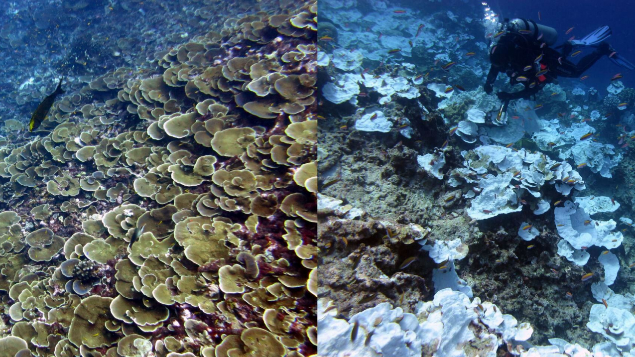
Make the inference visible before trusting it
A landscape can keep the same number of species at each site while losing the differences that make its communities distinct.
Biotic homogenisation is a directional increase in similarity among communities through time. It is not simply low diversity, urbanisation or the arrival of a widespread species. The gold standard compares matched places and periods, names the dimension of diversity and shows whether common winners are replacing distinctive losers.
Frame the claimROUTE 02 · CHAPTERS 4–6
Work the evidenceROUTE 03 · CHAPTERS 7–9
Test transferROUTE 04 · CHAPTERS 10–12
Audit and continue
Open the chapter contents · Visit the Ecology root
Chapter contents
01 · Frame the claim
02 · Work the evidence
03 · Test transfer
Two sites are biotically homogenising when their assemblages become more similar through time. The claim therefore needs at least two places, two times and a defined similarity or dissimilarity measure.
A single contemporary survey can show that sites are similar, but not that similarity increased. Historical records, resurvey data or defensible time-for-space designs are needed to support a directional claim.
Alpha diversity describes diversity within a site. Beta diversity describes differentiation among sites. Gamma diversity describes the wider regional pool. These dimensions can move in different directions.
Local richness can stay constant, or even rise through introductions, while beta diversity falls because the same widespread species appear everywhere and distinctive species disappear. Reporting richness alone misses this reorganisation.
Taxonomic homogenisation concerns species identities. Functional homogenisation concerns traits or ecological roles. Genetic homogenisation concerns variation within or among populations. One does not guarantee another.
State the data type, taxonomic resolution, abundance treatment and index. Presence–absence Jaccard similarity answers a different question from abundance-weighted Bray–Curtis dissimilarity, and trait-space overlap depends on the chosen traits and distances.
| Dimension | Unit | Example question |
|---|---|---|
| Taxonomic | Species identity or abundance | Are sites sharing more species? |
| Functional | Traits or roles | Are ecological strategies converging? |
| Genetic | Alleles or populations | Is within-region variation shrinking? |
Repeat the same spatial grain, season, survey duration, gear, time of day and detectability controls as closely as possible. A larger modern search effort will discover more common species and can falsely suggest convergence.
Reconcile scientific names, splits, lumping and identification standards before comparison. Retain an audit table from each historical name to the accepted analysis unit, including uncertain records and changes in taxonomic resolution.
Overall beta diversity can arise because sites contain different species—turnover—or because a poorer site is largely a subset of a richer one—nestedness. Similar total dissimilarity can therefore reflect different ecological processes.
Partitioning helps distinguish replacement from ordered loss, but the components remain descriptive until linked to colonisation, extinction, dispersal, land use or environmental filtering. Use the partition that matches the index and question.
| Component | Pattern | Possible process |
|---|---|---|
| Turnover | Replacement among sites | Colonisation and extinction |
| Nestedness | One assemblage becomes a subset | Ordered loss |
| Abundance shift | Same species, new dominance | Filtering or disturbance |
6. Worked example: richness holds while distinctness falls
At Time 1, Site A contains {a, b, c, d} and Site B contains {e, f, g, h}. They share no species, so Jaccard similarity is 0 divided by 8, or 0. At Time 2, Site A contains {a, b, x, y} and Site B contains {e, f, x, y}.
Each site still has four species, but the sites now share x and y. Their intersection is 2 and their union is 6, so Jaccard similarity is 2/6, or about 0.33. Local richness did not decline, yet the pair homogenised. The next question is whether x and y are widespread winners, whether c, d, g and h were lost, and whether effort was comparable.
Track species gained and lost at each site, then classify range expansion, introduction, local extinction and taxonomic uncertainty. Homogenisation often involves common generalists expanding while restricted specialists decline, but differentiation is also possible.
Use occupancy or detection models when observation probability varies. Test whether environmental convergence, connectivity, disturbance or propagule pressure predicts the change while respecting spatial dependence.
| Record | Contribution | Caution |
|---|---|---|
| Colonisation | New local occurrences | Detection may improve |
| Extinction | Lost local occurrences | Absence may be false |
| Range status | Restricted or widespread | Pool definition matters |
Move the design from plant species to urban pollinator traits. The time-by-site comparison transfers, but species identity is replaced by a functional representation such as body size, nesting strategy, diet breadth and activity season.
Trait databases may be incomplete or assign one value to variable populations. Functional homogenisation should therefore be checked across plausible trait choices and imputation rules, not inferred automatically from taxonomic convergence.
Homogenisation is not always a global monotonic trend. Sites can differentiate during invasion, recover distinctiveness after restoration or show taxonomic convergence with functional divergence. Results depend on grain, extent, time interval and index.
Do not call every increase in introduced species homogenisation. Do not infer process from one similarity number. Do not pool habitats with different sampling completeness or treat an unresolved species complex as the same taxon across decades without review.
Archive site coordinates, sampling polygons, survey effort, dates, raw detections, taxonomic crosswalk and the regional pool. Plot pairwise changes rather than only a regional average, because a few strongly converging pairs can drive the summary.
Repeat the analysis with presence–absence and abundance-sensitive measures, alternative rare-species rules, matched effort and plausible detection corrections. Report whether direction and magnitude remain stable.
| Check | Evidence | Failure signal |
|---|---|---|
| Temporal match | Same sites and seasons | Snapshot called change |
| Effort | Comparable detection process | Modern survey much stronger |
| Sensitivity | Indices and taxonomy rules | One metric decides result |
Can richness increase during homogenisation?
Yes. Local additions can increase alpha richness while the same additions make sites more alike and reduce beta diversity.
Is low beta diversity evidence of homogenisation?
Not by itself. Homogenisation is a temporal change toward lower differentiation; naturally similar sites may have low beta diversity without recent change.
Which similarity index is best?
No index is universally best. Choose one aligned to presence, abundance or traits, then test whether the conclusion depends on that choice.
12. The gold standard follows distinctness through time
Biotic homogenisation matters because a region can retain many organisms while losing ecological and evolutionary distinctness among places. The inference must show that resemblance increased and identify what entered, disappeared or changed in abundance.
Before accepting the claim, ask whether local richness was confused with beta diversity, whether turnover was separated from nested loss and whether survey comparability survives audit. Distinctness deserves measurement as carefully as richness.
Contents · Previous chapter · Ecology root · Return to Ecology
Continue through verified routes
Core route
- Ecology: subject root and specialist index
- The Gold Standard of Education: learning transfers into life
- The Gold Standard: eduKate Singapore
- How X Works: systems and first-principles hub
Specialist route
- Spatial grain, extent and scale-dependent patterns
- Edge effects, buffer width and boundary leakage
- Pseudoreplication, spatial autocorrelation and effective replication
- Observation effort, time-of-day windows and phenology mismatch
- Colonisation credit, extinction debt and delayed community response
Authoritative sources
- Olden and Rooney, Biotic homogenization and a conservation biogeography research agenda
- McKinney and Lockwood, A few winners replacing many losers
- Baselga, Partitioning turnover and nestedness components of beta diversity
- Olden and Poff, Ecological processes driving biotic homogenization
- Wayman et al., Unravelling the complexities of biotic homogenization