
Make the inference visible before trusting it
Joint models can borrow information across species and reveal residual co-occurrence, but a latent association is not automatically a biotic interaction.
Joint species distribution models analyse the responses of many species together. They can estimate species-specific environmental relationships, share information across taxa and describe residual association after measured covariates are included. Latent factors provide a parsimonious representation of that remaining structure, but they can absorb missing environment, spatial pattern, observation error and sampling design as well as ecological interaction.
Frame the claimROUTE 02 · CHAPTERS 4–6
Work the evidenceROUTE 03 · CHAPTERS 7–9
Test transferROUTE 04 · CHAPTERS 10–12
Audit and continue
Open the chapter contents · Visit the Ecology root
Chapter contents
01 · Frame the claim
02 · Work the evidence
03 · Test transfer
Decide whether the aim is prediction, environmental response, ordination, community turnover, rare-species borrowing or residual association. These aims favour different likelihoods, hierarchies and validation targets. A model chosen because it returns an association matrix may answer the wrong ecological question. Define the sampling unit, response scale and prediction domain before choosing a framework.
Presence–absence, counts, biomass and percentage cover have different observation processes. Choose Bernoulli, Poisson, negative-binomial, hurdle, ordinal or compositional structures that match how data were generated. Overdispersion, excess zeros and detection error do not vanish when species are modelled jointly. A poorly fitted marginal model can manufacture cross-species residual structure.
3. Separate measured environment from residual structure
The fixed part of a JSDM estimates how each species responds to recorded covariates. Residual association describes covariance left after those predictors and other model components. Positive residual association means species co-vary beyond the fitted explanation; negative association means they separate. Neither label supplies a mechanism. Omitted habitat, shared dispersal, observer effects and direct interaction can produce similar signs.
| Model component | Explains | If omitted |
|---|---|---|
| Environmental predictors | Measured niche response | Habitat becomes residual association |
| Observation process | Detection and sampling variation | Error resembles ecology |
| Residual covariance | Remaining co-variation | Species treated as conditionally independent |
A small number of latent variables can represent patterns shared by many species without estimating every covariance freely. Species loadings describe how each taxon relates to those latent dimensions. The factors may act like unmeasured gradients or a regularised ordination device, but their axes can rotate and their biological meaning is not guaranteed. Choose factor number through predictive checks and sensitivity, not a visually pleasing biplot.
5. Put space, time and hierarchy where they belong
Residual association can arise because nearby sites share unmeasured conditions or because surveys recur through time. Spatially structured latent factors, site random effects and temporal components can reduce confounding, but they introduce scale and prior choices. Include sampling hierarchy—plots within sites, visits within seasons—rather than letting one latent layer carry every source of dependence.
| Dependence source | Useful component | Caution |
|---|---|---|
| Nearby habitat | Spatial latent factor | May confound spatial covariates |
| Repeated surveys | Temporal or site effect | Needs time scale |
| Observer or gear | Effort and observer effect | Not a biological association |
6. Worked example: woodland birds across 80 plots
A presence–absence JSDM includes canopy cover, elevation and distance to water for 22 bird species. Two insectivores retain a positive residual association. Adding a spatial latent factor weakens it, and adding observer identity weakens it further; prediction improves at held-out plots. The study reports shared unmeasured spatial habitat or observation as the leading explanation, not facilitation. A targeted food survey and repeated detection design are proposed before any interaction claim.
Randomly splitting observations can leak spatial or temporal dependence into both training and test sets. Use site-blocked, spatially separated or forward-in-time validation that matches the intended transfer. Assess calibration and discrimination for species, but also community summaries and joint predictions. A model can predict common species well while failing rare taxa or the covariance pattern that motivated joint modelling.
| Validation split | Tests | Leakage risk |
|---|---|---|
| Random records | Interpolation among observations | Nearby sites in both sets |
| Spatial blocks | New locations | Block size mismatch |
| Forward time | Future surveys | Changing effort or climate |
8. Changed-context transfer check: reef recovery after bleaching
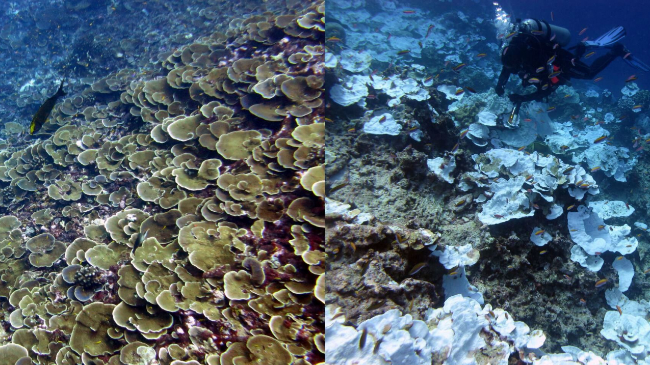
A reef JSDM models coral and fish assemblages before and after bleaching. The transferable rule is to separate measured environmental response from residual association. The context adds compositional cover, imperfect fish detection and a strong shared disturbance. A new negative association after bleaching could reflect constrained space, differential survival or survey conditions; causal competition requires process evidence beyond the fitted covariance.
JSDMs do not solve causal inference merely by modelling species together. Residual correlations are conditional on the chosen covariates, scales, likelihood and random effects. Latent variables are not directly measured environmental gradients. More factors can fit noise, while too few can leave structure. Borrowing strength can help rare species but may pull genuinely unusual responses toward a community mean. Predictions beyond sampled environments remain extrapolations.
10. Audit data, model and ecological interpretation
Publish the community matrix, effort variables, taxonomic decisions, covariates, transformations, spatial coordinates, hierarchy, priors, factor choices and code. Inspect posterior predictive checks or residual diagnostics by species and site. Repeat the analysis with alternative likelihoods, factor counts, spatial structures and covariate sets. Report which associations persist and which disappear when plausible missing structure is represented.
| Audit layer | Retain | Failure signal |
|---|---|---|
| Data | Matrix, effort and covariates | Zeros assumed equal |
| Model | Likelihood, priors and factors | Defaults unreported |
| Inference | Sensitivity and rival mechanisms | Correlation named as interaction |
Is a positive residual association facilitation? No; it is compatible with several mechanisms. How many latent factors are needed? Enough for the intended predictive and residual structure, judged with diagnostics and sensitivity. Can rare species benefit? Yes, through hierarchical sharing, provided shrinkage is checked. Must the model be Bayesian? No; several likelihood-based and Bayesian JSDM frameworks exist.
12. The gold standard keeps association conditional
Joint models become valuable when they clarify what many species share and where their responses differ. The gold standard fits the observation process, represents space and hierarchy, validates the intended task and treats latent factors as conditional summaries. Residual association is evidence that the fitted explanation is incomplete—not automatic proof of the ecological mechanism that completes it.
Contents · Previous chapter · Ecology root · Return to Ecology
Continue through verified routes
Core route
- Ecology: subject root and specialist index
- The Gold Standard of Education: learning transfers into life
- The Gold Standard: eduKate Singapore
- How X Works: systems and first-principles hub
Specialist route
- Detection probability, repeat surveys and false absence
- Spatial grain, extent and scale-dependent patterns
- Pseudoreplication, spatial autocorrelation and effective replication
- Metacommunity dynamics, dispersal limitation and mass effects
- Null models, species co-occurrence and checkerboard patterns