
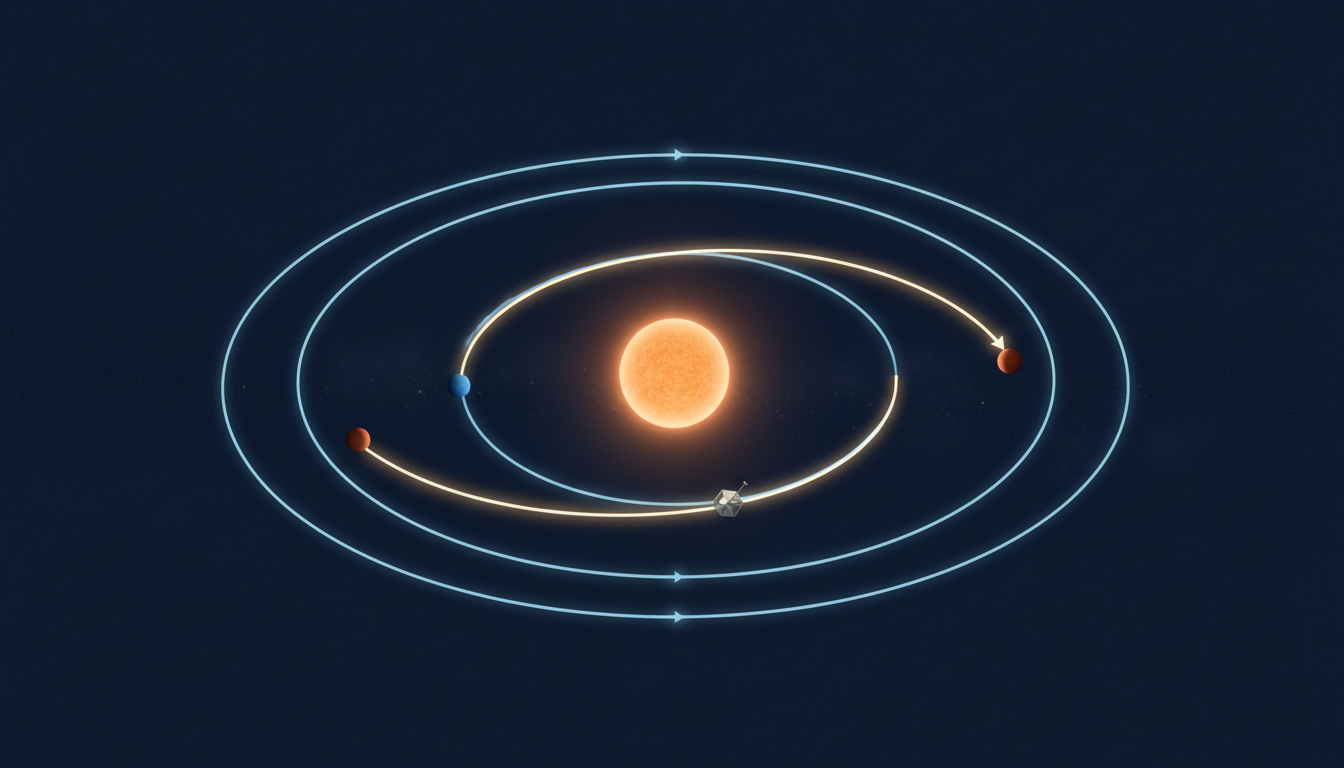
An interplanetary spacecraft must intercept a planet that keeps moving while the spacecraft is travelling. The path must also account for gravitational forces, propulsion, navigation uncertainty and the energy needed to arrive in a useful condition.
The Gold Standard of Interplanetary Dynamics begins with fundamental physics, uses transparent approximations to explain transfers, and then shows why mission teams refine the resulting trajectories with observations and robust models. The aim is a path that remains defensible when the real solar system refuses to behave like a static textbook drawing.
This reference contains 29 guided chapters, three checked fictional or idealised calculations, operational diagnostics, frequently asked questions and direct NASA and JPL reading routes.
Chapter index
Foundations, ephemerides and transfer windows · Chapters 1–11
- Interplanetary dynamics is a moving-target problem
- Gravity supplies the dominant acceleration
- Reference frames and time standards must be named
- Two-body trajectories create the starting model
- Energy links speed to distance and orbit size
- Angular momentum explains orbital geometry
- Conic sections represent different mission phases
- Use ephemerides instead of fixed planetary dots
- Worked example: an idealised Earth-to-Mars transfer time
- A transfer must match the arrival time and phase
- Worked example: approximate launch-window recurrence
Trajectory design, encounters and navigation · Chapters 12–23
- Patched conics join useful local approximations
- Launch energy and departure geometry constrain missions
- Sphere-of-influence models are design conveniences
- Encounter design includes altitude and geometry
- Gravity assists exchange momentum with a moving planet
- Rendezvous and capture differ from a simple flyby
- Atmospheric braking changes the energy balance
- Low-thrust trajectories require another design style
- Navigation combines physics with measured radio signals
- Orbit determination must expose uncertainty
- Midcourse manoeuvres correct the planned path
- Worked example: keep manoeuvre budget and margin distinct
Budgeting, perturbations, validation and deeper learning · Chapters 24–29
- Small perturbations matter over long cruises
- Planetary protection can constrain navigation corridors
- Launch windows are multidimensional trade-offs
- Validate models with independent checks and Monte Carlo tests
- Frequently asked questions about interplanetary dynamics
- Continue through the Gold Standard scientific roots
1. Interplanetary dynamics is a moving-target problem
Interplanetary dynamics concerns the motion of spacecraft and celestial bodies under gravity, propulsion and smaller environmental forces. A mission does not aim for the location where a planet appears at departure. It must design a path that reaches the planet’s future position under constraints on launch vehicle capability, propellant, time, safety and navigation accuracy.
The gold standard is not the most elegant orbit drawn on a diagram. It is a trajectory that can be reproduced from specified assumptions, tested against realistic perturbations, navigated with observations and adjusted safely in flight. Mission success depends on the entire arrival condition, including velocity and approach geometry, not simply intersecting the destination’s orbital distance.
2. Gravity supplies the dominant acceleration
Newtonian gravity provides a powerful first model. For a point-like central body with gravitational parameter μ = GM and distance r, acceleration magnitude is μ/r² toward the centre. Here G is the gravitational constant and M is the body’s mass. Position and velocity together determine the spacecraft’s subsequent path under the chosen force model.
A higher-fidelity design includes the attraction of multiple bodies and sometimes radiation pressure or relativistic terms. Treat μ as a parameter with units of distance cubed per time squared, and keep a consistent unit system. An equation copied without units or an explicit central body can produce a numerically convincing but physically wrong trajectory.
3. Reference frames and time standards must be named
A vector makes sense only in a specified reference frame, origin and epoch. Earth-centred inertial coordinates, heliocentric positions, planet-fixed maps and a spacecraft’s local orbital frame serve different tasks. Translating between them requires the applicable transformations and rotation model; an altitude relative to a surface is not an absolute distance from the planet’s centre.
Report times with an explicit time scale, calendar convention and relevant light-time treatment. A few seconds of timing error can shift a fast-moving encounter substantially. The JPL Horizons manual documents operational choices for precise planetary and spacecraft ephemerides.
4. Two-body trajectories create the starting model
If one massive central body dominates and the spacecraft exerts negligible influence, ideal two-body motion follows a conic section. Bound negative-energy orbits are ellipses, the circular case is a special ellipse, and unbound paths are parabolic or hyperbolic. The model links geometry, energy and time without integrating every particle in the solar system.
This simplification is valuable for deriving transfer ideas and checking software, but it is not a promise that the solar system has only two gravitating objects. Near planetary encounters or over long cruise intervals, third-body effects and other perturbations may require numerical integration.
5. Energy links speed to distance and orbit size
In the ideal two-body model, the vis-viva equation is v² = μ(2/r − 1/a), where v is speed, r is instantaneous distance from the centre and a is the conic semimajor axis for an elliptical orbit. It explains why a spacecraft moves faster near periapsis and slower near apoapsis in a bound eccentric orbit.
Interpret the quantities with care: changing v through a burn changes the orbit, and a transfer segment can require a different central body from a planet-relative arrival arc. Do not apply a Sun-centred velocity directly as if it were a Mars-relative approach velocity. Check reference frames before comparing numerical results.
6. Angular momentum explains orbital geometry
The specific angular momentum vector is the cross product of position and velocity relative to the selected central body. In a pure two-body field it remains constant, and the motion stays in one orbital plane. This gives a powerful consistency check for approximate calculations and helps explain why orbital-plane changes can be expensive.
Real burns and noncentral forces alter the vector. In mission design, inclination, line of nodes and encounter geometry affect where and when a trajectory can connect to another body’s orbit. A low-energy transfer in a simplified plane may be useless if the actual destination geometry requires a costly change in direction.
7. Conic sections represent different mission phases
An ellipse may represent a heliocentric transfer or a captured planetary orbit. A hyperbola often describes an approach or departure relative to a planet when the spacecraft’s excess speed remains positive far from that planet within a simplified model. Different conic sections can describe adjoining portions of the same mission.
Specify periapsis, apoapsis where defined, eccentricity and excess velocity with the relevant central body. A hyperbolic excess speed is not the same as the spacecraft’s instantaneous speed during closest approach. Labels such as ‘escape velocity’ need the location and frame to be meaningful.
8. Use ephemerides instead of fixed planetary dots
Planets and moons move, their orbits are not perfect circles and their positions must be evaluated at particular times. An ephemeris supplies calculated positions and velocities according to a stated dynamical model and time range. It is therefore a core input to trajectory searches, targeting and interpretation of tracking observations.
JPL Horizons provides observer tables, vector tables and orbital elements for solar system objects. Record the requested body, observer centre, frame, epoch, output units and source version. Reproducibility fails when a plot carries none of these settings.
9. Worked example: an idealised Earth-to-Mars transfer time
Take fictionalised circular coplanar Sun-centred orbits at 1.000 AU for Earth and 1.524 AU for Mars. A Hohmann-style ellipse tangent to both has semimajor axis a = (1.000 + 1.524)/2 = 1.262 AU. With Kepler’s third-law scaling T² = a³ when years and AU are used relative to Earth’s orbit, the transfer ellipse’s period is approximately √(1.262³) = 1.417 years.
The outward half of the ellipse takes about 1.417/2 = 0.709 years, or roughly 259 days. This is a teaching approximation, not a flight plan or a claim about a specific Mars mission. It omits actual planetary eccentricity and inclination, departure energy, launch dates, correction manoeuvres and capture requirements. NASA’s trajectory primer explains the Hohmann-transfer idea.
10. A transfer must match the arrival time and phase
Reaching Mars’s orbital radius is not the same as reaching Mars. The planet continues moving while the spacecraft travels. A departure opportunity exists when the planets have an angular relationship that permits a useful transfer for the chosen duration and energy. The spacecraft is targeted toward a future intercept state, not a static dot.
Planners search launch dates and arrival dates together, often trading propulsion requirements against travel time and arrival conditions. A diagram should label the departure and encounter epochs; without them the geometry alone cannot establish whether the transfer is feasible.
11. Worked example: approximate launch-window recurrence
Assume for illustration that Earth’s orbital period is 1.00 year and Mars’s is 1.88 years. Their relative orbital frequency is |1/1.00 − 1/1.88| cycles per year. The synodic period is therefore approximately 1 ÷ (1 − 1/1.88) = 2.14 years, or about 25.6 months.
This is the approximate repetition of relative orbital geometry, not a guarantee that every opportunity has identical energy, spacecraft constraints or weather. Real launch windows vary with eccentric orbits, mission objectives and operations. NASA describes low-energy Earth–Mars opportunities as recurring roughly every 25 months, consistent with this simplified calculation.
12. Patched conics join useful local approximations
An early design can approximate departure around Earth with an Earth-centred trajectory, cruise around the Sun with a heliocentric trajectory and arrival around Mars with a Mars-centred trajectory. The connecting velocities and geometry must agree at the handoffs. This patched-conics method is useful for concept studies and first estimates.
The patches do not imply a sharp physical edge where one planet’s gravity switches off. Real gravity fields overlap continuously. Refine promising candidate paths with numerical propagation under several bodies before relying on them for navigation or mission commitments.
13. Launch energy and departure geometry constrain missions
An interplanetary launch is commonly characterised in part by the spacecraft’s hyperbolic excess speed relative to Earth, and C3 is the square of that speed. C3 has units of squared speed, not energy per unit spacecraft in the everyday accounting sense. The launch vehicle’s available performance depends on payload mass and the departure conditions.
An Earth-escape calculation and a heliocentric transfer must be connected consistently. A departure burn that points in the wrong direction can waste energy even if its magnitude is large. Consider launch-site, parking orbit, injection accuracy and mission geometry rather than assuming any sufficiently powerful rocket works on any day.
14. Sphere-of-influence models are design conveniences
The sphere-of-influence concept helps decide when a planet-centred approximation is useful in a patched-conics calculation. It is not a membrane or a boundary between gravity and no gravity. A spacecraft remains influenced by the Sun, the planet and other bodies at all distances.
During close encounters the planet-relative trajectory may dominate the geometry, while long interplanetary cruise often uses a Sun-centred reference. Full-force numerical models can avoid an artificial handoff altogether. The best model is the simplest one whose errors remain acceptable for the decision being made.
15. Encounter design includes altitude and geometry
A flyby must meet a particular aim point and approach asymptote, not merely pass near a planet. Closest-approach altitude affects gravitational deflection, observation opportunities and hazards; too low an approach may encounter atmosphere or terrain, while too high may not produce the desired turn.
Define the encounter using a suitable target-plane or B-plane description where applicable. Include navigation covariance, body size, atmospheric uncertainty and instruments’ line-of-sight requirements. A mathematically reachable point can still be an unsafe or scientifically unproductive encounter.
16. Gravity assists exchange momentum with a moving planet
During a flyby, planetary gravity bends a spacecraft’s velocity vector relative to the planet. In a Sun-centred frame, the spacecraft’s orbital energy may increase or decrease because the planet is moving. This exchange enables mission architectures that could demand much larger propulsive changes if attempted entirely with engines.
It is misleading to describe the spacecraft as getting free energy from gravity without a reference frame. Planet-relative ideal flyby speed far before and after is approximately the same, while the heliocentric speed can change. NASA’s trajectories chapter explains this frame-dependent momentum exchange.
17. Rendezvous and capture differ from a simple flyby
A spacecraft can pass through a target’s region at high relative speed without staying there. Orbit insertion or rendezvous requires a suitable reduction or shaping of relative energy through propulsion, atmospheric forces or other mission-specific methods. A low flyby altitude is not itself proof that capture has occurred.
Estimate the arrival excess speed, target orbital geometry and required manoeuvre, then check whether the spacecraft can supply it with reserves. A sample-return mission or lander adds further operations, including departure from the target and potentially Earth entry. Mission constraints must be evaluated across the whole journey.
18. Atmospheric braking changes the energy balance
A planetary atmosphere can help reduce speed, enabling aerobraking or entry systems that save propellant for suitable destinations and vehicles. Such methods introduce sensitivity to atmospheric density, heat flux, structural loads, guidance capability and uncertain weather or dust conditions.
Do not apply an ‘atmospheric capture’ assumption to a body without a suitable atmosphere. Mission designers compare propulsion, aeroshell mass, thermal protection, science constraints and navigation risk. An energy-saving technique is not automatically the safest or lowest-cost approach after system-level trade-offs.
19. Low-thrust trajectories require another design style
Electric or other low-thrust systems can apply small accelerations over extended periods rather than brief high-thrust impulses. Their trajectories may spiral, change energy gradually and require optimisation of thrust direction, power, duty cycle and total mission time. A short impulsive Hohmann calculation is not enough to describe such a mission.
Use a dynamic model that couples orbit propagation to thrust and spacecraft mass where necessary. Check periods of eclipse, power availability and communication constraints. NASA’s primer contrasts low-thrust ion propulsion with shorter chemical-rocket manoeuvres.
20. Navigation combines physics with measured radio signals
Real trajectories drift from the reference because initial conditions, unmodelled forces and propulsion execution are uncertain. Mission teams use radiometric tracking and, where available, optical observations to estimate the spacecraft’s state. Range and Doppler constrain different aspects of motion, and a dynamics model connects observations across time.
NASA’s navigation chapter explains orbit determination using range, line-of-sight velocity and optical measurements. Reporting a spacecraft’s position without an epoch, frame and uncertainty is incomplete.
21. Orbit determination must expose uncertainty
A navigation solution estimates position and velocity from imperfect observations. Error sources include measurement noise, station geometry, force-model inaccuracies, timekeeping and manoeuvre uncertainty. A covariance description can summarise uncertainty under model assumptions, but it should not be mistaken for a guarantee that all errors are Gaussian or fully represented.
Check residuals against independent observations, monitor systematic biases and validate the trajectory with alternative techniques when practical. A beautifully smooth propagated curve can still be wrong if its initial state or gravitational parameters were estimated incorrectly.
22. Midcourse manoeuvres correct the planned path
Small burns may adjust arrival timing and geometry after navigation updates. Mission designers plan manoeuvre opportunities, expected magnitude, propellant allowance, commanding lead time and the ability to recover from an under- or over-executed burn. A planned correction is not automatically evidence that the initial design failed.
Compare the estimated state with the target corridor and evaluate whether the proposed manoeuvre reduces overall risk. The best correction is not necessarily the one that eliminates every observed error immediately: errors may be correlated or expected to shrink after further tracking.
23. Worked example: keep manoeuvre budget and margin distinct
Consider a fictional mission with planned delta-v allocations of 3.1 km/s for injection, 0.1 km/s for correction opportunities and 1.2 km/s for capture. The sum is 4.4 km/s. If designers assign a 20% planning margin to this simplified total, the additional allowance is 0.88 km/s and the illustrative budget becomes 5.28 km/s.
Delta-v is a bookkeeping measure of required velocity change across burns; it is not automatically convertible to one propellant mass without a mass model, propulsion performance and burn sequencing. Do not treat these example values as actual Earth-to-Mars mission requirements. The point is to show every included manoeuvre and separately label the margin.
24. Small perturbations matter over long cruises
Solar radiation pressure, non-spherical gravity, third-body forces and spacecraft outgassing can shift a trajectory. Their importance depends on spacecraft area-to-mass ratio, trajectory duration and required navigation accuracy. A force too small to matter during one hour may become important during months of cruise.
NASA’s Ames trajectory-design guidance describes high-fidelity models that include multiple gravity fields, solar radiation pressure and statistical simulations. Select the forces needed for the decision rather than blindly adding complexity without validation.
25. Planetary protection can constrain navigation corridors
A trajectory near a body of astrobiological interest may require controls to reduce the risk of unintended impact or microbial contamination. Forward contamination concerns organisms carried from Earth to other bodies; return missions raise distinct backward-contamination issues. Requirements depend on target and encounter type.
NASA’s planetary-protection guidance makes clear that avoidance of unintended encounters can be a mission-design requirement. A lower propellant trajectory is not automatically admissible if it violates protection, safety or mission-assurance constraints.
26. Launch windows are multidimensional trade-offs
Mission planners balance launch date, launch vehicle capability, flight duration, encounter speed, planetary phase, thermal and communication geometry, arrival conditions and risk. A low-energy candidate may take too long or reach the destination with unacceptable speed. Higher-energy options can trade propellant for timing, but may violate payload or mission limits.
Use a grid of departure and arrival dates to explore the feasible region, then refine interesting candidates. Label any plot’s axes and units. A coloured ‘porkchop’ launch plot is useful only when the reader knows which measure it represents and which constraints were excluded.
27. Validate models with independent checks and Monte Carlo tests
Begin with simple analytic approximations that reveal orders of magnitude, then compare them with numerical integration and authoritative ephemerides. Check energy or angular momentum conservation where their assumptions apply. Verify frames, time standards, force models, event detection, interpolation and the exact spacecraft mass profile.
To estimate operational robustness, vary plausible initial-state errors, burn execution, atmospheric properties and measurement noise across simulated trials. Report the input distributions and which outcomes count as success. A nominal path that works once is not enough if reasonable uncertainty makes many simulated outcomes unsafe.
28. Frequently asked questions about interplanetary dynamics
Does a spacecraft travel in a straight line to Mars? No, it follows a path shaped by gravity and any propulsion. Is Hohmann transfer always the fastest route? No; it is a useful two-body low-energy reference, not a universal minimum-time solution. Does a gravity assist create energy? Its heliocentric energy change results from momentum exchange with a moving planet.
Does reaching a planetary orbit mean reaching the planet? No; timing and encounter velocity must match. Is the 259-day teaching example a promised Mars travel time? No. Can a strong tracking signal prove the spacecraft is on course? It contributes measurements; state estimation and uncertainty analysis establish the navigation solution.
29. Continue through the Gold Standard scientific roots
Interplanetary dynamics connects Physics, Astronomy, Aerospace Engineering, Jet Propulsion, Mathematics and Statistics. Each contributes a different piece of a reproducible trajectory and its evidence.
Primary references include NASA Trajectories, NASA Navigation, JPL Horizons, NASA Ames trajectory design and NASA planetary protection. All numerical examples are simplified educational illustrations, not launch guidance or real spacecraft command instructions.