
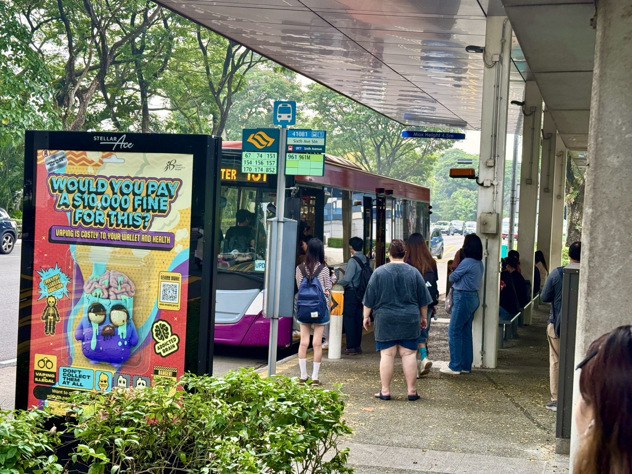
The gold standard of queueing theory is a model that connects arrivals, available service and waiting under explicit assumptions. It defines the system boundary, counts the right population and checks both average and difficult experiences. A shorter queue becomes a useful result when work is completed well and people retain fair access.
Queueing theory explains a familiar puzzle: a service can have more average capacity than demand and still produce long waits. Variability, peak arrivals, service-time differences and routing shape what happens through time. The same questions appear in call centres, elevators, websites, work queues and requests for educational help.
This root guide connects eduKate’s existing queueing articles with worked examples, measurement checks and onward routes. Numerical cases are hypothetical teaching examples. Simple stationary models are explanatory baselines, not staffing instructions, safety assessments or promises about a particular service.
Find the part you need
Choose a task, or read from the beginning. The teaching chapters stay open.
Chapter index
Chapters 1–4
Chapters 5–8
Chapters 9–12
Chapters 13–16
Chapters 17–18
The gold standard of queueing theory is a model that states who or what arrives, which resource provides service, how waiting is organised and what outcome matters. A queue may contain people, calls, repair jobs, data requests, vehicles or unfinished work. It need not be a visible line.
The first decision is the system boundary. Does a visitor enter the system on arrival at a building, at check-in or at a service desk? Does time end at first contact or at completion? Different boundaries produce different valid measurements, but they cannot be mixed.
Imagine a hypothetical help desk. A person spends five minutes filling in a form, ten minutes waiting and four minutes speaking with a member of staff. The waiting-line time is ten minutes, while the full journey from form start is nineteen minutes. Neither number replaces the other.
A useful explanation also states the purpose. Reducing average waiting, preventing very long waits, maintaining access and preserving service quality can lead to different choices. A model should expose those choices rather than hide them behind one efficiency score.
The existing queueing theory and waiting-times guide provides the foundation. This root connects it with the wider applications and evidence questions across eduKate’s ecosystem.
A queue has an accounting identity before it has a probability model. For a defined system, the number present at the end equals the number present at the start plus entries minus exits, provided every relevant movement is included.
Suppose a fictional support service begins an hour with 12 open requests, admits 30 more and closes 25. It ends with 17 open requests if there are no other entries, exits or reclassifications. This is a flow balance, not a forecast of individual waiting times.
Requests closed are not necessarily problems solved. A duplicate merge, rejected request or abandoned case may also leave the measured system. The operational record should distinguish these outcomes if the purpose is to understand access and resolution.
The same person can generate several contacts. Decide whether the unit is a person, a visit, a call attempt or a work item. A reduction in open tickets can coexist with more unresolved people if the counting unit changes.
Begin an analysis by checking that the event records reconcile. A sophisticated waiting-time formula cannot repair missing departures or a boundary that moves halfway through the observation.
An average arrival rate λ of 12 jobs per hour corresponds to a mean spacing of five minutes, but it does not mean that a job arrives exactly every five minutes. Bunching can create waiting even when the average workload appears manageable.
A homogeneous Poisson arrival model assumes independent increments and a constant rate. Under that model, counts over an interval have a Poisson distribution, and interarrival times are independent exponential random variables. Those are assumptions about a process, not consequences of any average count.
School dismissal, a train unloading, a sale opening or a software retry burst can create dependent or time-varying arrivals. A daily total hides this pattern. Plot counts against time before choosing a stationary model.
EduKate’s Poisson processes guide connects the count and waiting-time views. It also explains why a familiar distribution is useful only when its structural assumptions fit the question.
For an invented comparison, 60 arrivals spread evenly over an hour and 60 arrivals within its first five minutes have the same hourly count. Their immediate capacity requirements and waits can be very different. The time pattern belongs in the model.
If the mean service time of one continuously available server is six minutes, its reciprocal service rate μ is ten jobs per hour. Convert units before taking the reciprocal. Six minutes is 0.10 hour, so μ = 1/0.10.
Availability matters. A person scheduled for eight hours is not necessarily available to serve continuously for eight hours. Breaks, training, setup, documentation and interruptions need explicit definitions in the workload model.
Service times can also vary widely. Two systems may share the same mean while one has mostly similar jobs and the other has a mixture of short and very long jobs. The second pattern can have a different waiting distribution.
Do not assume that a completed job’s elapsed time is all active processing. It may include waits for information, approvals or another resource. Separating these intervals can identify a coordination problem that additional front-desk staffing would not fix.
Report the service-time distribution and effective availability alongside the average. The purpose is to understand how work is completed, rather than to treat a person as a machine with one permanently fixed speed.
For a basic single-server queue, utilisation is ρ = λ/μ. With six arrivals per hour and capacity of eight per hour, the ratio is 0.75. In the stable, work-conserving model without losses, the server is busy for a long-run fraction 0.75 of the time.
The ratio is not the probability that any particular person receives immediate service in every kind of queue. That interpretation requires further assumptions about arrivals and the model. Nor is it a complete measure of staff effort or service quality.
For the standard M/M/1 queue with positive rates and an unlimited waiting room, a stationary distribution requires λ < μ. At or above equality, the usual finite steady-state mean waiting formulas are unavailable.
A finite-capacity queue can avoid an unbounded count by rejecting arrivals. That changes the outcome rather than proving that demand is adequately served. A bounded queue and a satisfactory service are different claims.
Spare capacity is therefore not automatically waste. It can provide room for variability, disruption and recovery. The appropriate margin depends on the task, evidence and consequences; there is no universal percentage that solves every waiting problem.
The standard M/M/1 model has Poisson arrivals, independent exponentially distributed service times, one server, an unlimited waiting space and stable operation with λ < μ. Use first-come service for the waiting-time interpretation here, with no abandonment or retries.
Let λ = 6 per hour and μ = 8 per hour. The stationary mean time in the system is W = 1/(μ − λ) = 0.50 hour, or 30 minutes. Mean service time is 1/μ = 7.5 minutes.
Mean waiting before service is Wq = W − 1/μ = 22.5 minutes. The average number in the system is L = λW = 3, while the average number waiting is Lq = λWq = 2.25.
The fractional average is meaningful. There are whole jobs present at each instant, but the average over time can be 2.25. Also, L includes the job being served, whereas Lq excludes it.
The MIT M/M/1 teaching note distinguishes these quantities. These invented rates produce a model result, not a prediction for every desk with the same average load.
Keep the same M/M/1 service rate μ = 8 per hour but increase arrivals from 6 to 7 per hour. Mean system time becomes 1/(8 − 7) = 1 hour. Mean waiting becomes 52.5 minutes after subtracting the 7.5-minute mean service time.
Arrivals rose by one sixth, while the model’s mean system time doubled. The denominator contains spare service capacity, μ − λ, so waiting grows nonlinearly as demand approaches capacity.
Now compare λ = 7.5 per hour with the same server. Mean system time is two hours and mean waiting is 112.5 minutes. That extreme sensitivity is a warning about operating close to the model’s stability boundary.
These are long-run stationary averages. A short service window that starts empty may behave differently, and real people may leave or be redirected. The model explains a mechanism without guaranteeing the same numerical result in a time-limited operation.
A useful planning question is how conclusions change when the estimated arrival or service rate shifts slightly. Sensitivity analysis is especially valuable near a boundary, where a small estimation error can produce a large change in predicted waiting.
Little’s Law relates compatible long-run averages through L = λW: average number in the defined system equals the effective entry rate multiplied by average time spent there. The limits and population must be well defined.
For a hypothetical service admitting 24 cases per hour, with mean time from entry to exit of 20 minutes, W is one third of an hour. The corresponding average number in the system is 24/3 = 8 cases.
For the waiting area alone, a suitable definition gives Lq = λWq. If every admitted case proceeds to service and mean waiting is five minutes, the average number waiting is 24 × 5/60 = 2.
Karl Sigman’s Columbia notes on Little’s Law explain its broad sample-path foundation. It does not require every system to have Poisson arrivals or exponential service times.
Use the entry rate for the population whose time is measured. If rejected attempts never enter, they do not belong in that system’s entry count. If admitted users abandon, their time until exit must be handled consistently rather than silently removed from one average but retained in another.
Mean demand and mean service capacity do not fully specify a waiting system. The spread of interarrival and service times matters, as does dependence between events. Long jobs can delay many later arrivals.
A coefficient of variation is standard deviation divided by mean. Squaring it gives a dimensionless measure often used in queueing approximations. A constant duration has zero variation; an exponential duration has coefficient of variation one.
The MIT basic queueing note presents a general-arrival, general-service single-server approximation that makes variability, utilisation and service time visible as separate influences.
That does not license replacing a whole distribution with a coefficient in every application. Correlated arrivals, heavy tails, priorities and nonstationary conditions can require richer analysis. An approximation should be checked against the decision and data.
Reducing avoidable variation can help without rushing the useful service. Complete information, reliable equipment and fewer repeated handoffs may stabilise work. Measure whether the change actually removes variability or simply moves difficult cases elsewhere.
A common queue feeding several eligible servers can reduce the chance that one server is idle while another line contains waiting work. Pooling creates a shared resource, but its benefits depend on what each server can actually do.
Compare two hypothetical desks with separate lines against one shared line. If both desks serve every job type equally well, a shared queue can use available capacity more flexibly. If one desk handles specialist work, routing needs to preserve that capability.
Two servers each completing six jobs per hour are not generally equivalent to one server completing twelve per hour. The service-time scale and number of simultaneous jobs differ, even though total nominal capacity matches.
Human factors also matter. Accessibility, privacy, travel distance, visible order and the effort of switching lines can influence the useful design. Pooling is a structural option rather than a promise of universal improvement.
Use The Gold Standard of Operations Research to connect the queue model with wider resource-allocation decisions. The objective and constraints should remain visible.
The Erlang C baseline models Poisson arrivals, independent exponential handling times, identical parallel servers, a first-come queue, unlimited waiting capacity and no abandonment. Stable operation requires offered load below the number of servers.
Offered load is a = λh, where h is mean handling time in the same time unit as the arrival rate. At 24 calls per hour and five minutes per call, a = 2 erlangs. This is average simultaneous workload, not a staffing recommendation.
With three continuously available identical agents, the baseline occupancy is 2/3. For this small Erlang C example, the probability of waiting is 4/9. Mean waiting is C h/(c − a), giving (4/9) × 5/(3 − 2) ≈ 2.22 minutes.
That average includes calls that wait zero. It is not the average only among delayed calls, nor a guarantee to the next caller. Real planning must account for skills, availability, changing demand, abandonment and the intended service definition.
The existing call centres and Erlang C guide develops the calculation and its limits. Use the model as a checkable baseline before deciding whether its assumptions fit.
First-come, first-served makes arrival order visible, but it is not the only queue discipline. Priority, appointments, deadlines and job-size rules can change waiting distributions and the experience of different groups.
A non-preemptive priority rule lets current service finish before selecting the next priority job. A preemptive rule can interrupt work in progress. That distinction affects both the model and the practical consequences.
Serving short jobs first can reduce some average completion measures under suitable assumptions, while making long jobs wait much longer. An attractive aggregate average can therefore coexist with an unacceptable outcome for one group.
Priority decisions need a stated purpose and safeguards against indefinite postponement. Queue mathematics can describe consequences, but it cannot by itself decide what counts as fair access or acceptable delay.
Keep service quality in the objective. A policy that makes a reported queue shorter by turning away complicated cases has changed access, not simply improved the original process. Measure both the waiting and what happens to the people or jobs affected.
Someone may decide not to join, join and later leave, or return after failing to get service. These behaviours change the relationship between offered demand, admitted demand and completed service.
A call centre with many abandoned calls can report a low average wait among answered calls. That does not establish good access. The result excludes people whose experience may be the reason the service needs attention.
A digital request that retries can create additional work. Under congestion, retries can increase arrivals further and amplify the original overload. Counting only unique users misses that workload; counting attempts alone can hide the user outcome.
State the denominator for every metric. Is the fraction answered within a target measured among all attempts, admitted contacts or completed contacts? Are immediate rejections and later abandonments included?
The existing message queues and delivery-guarantees guide connects waiting with acknowledgements, retries and processing. A drained queue does not prove that every intended task was completed correctly.
Many systems contain several stages. A quick first stage can feed work into a slow second stage, producing a downstream backlog. Improving one local queue does not automatically improve the full journey.
Elevators also move batches of people rather than acting as independent single-person servers. Travel, intermediate stops, direction, boarding and capacity interact. A simple M/M/1 formula is not a full elevator model.
Use the existing elevator dispatching guide and elevator motion and queueing guide to distinguish motion time, waiting and dispatch decisions.
For a hypothetical workflow, admission, review and approval form three stages. If reviews finish faster but approvals remain unchanged, completed reviews can accumulate. The relevant bottleneck may move after an improvement.
Measure the full system as well as each stage. A person may spend less time in a visible line but more time waiting for the next decision. System boundaries protect the meaning of any claimed improvement.
Processors, servers and distributed applications handle work through queues even when users see only a loading icon. Waiting can arise before execution, during access to shared resources or between services.
The CPU scheduling guide connects work ordering with response time. The load-balancing and tail-latency guide examines how work is distributed.
Tail latency describes the slower end of the response-time distribution. A system’s mean can improve while its 95th or 99th percentile remains poor. Report the sample, percentile definition and whether failed or timed-out work is included.
An overloaded service may need admission control, backpressure or different scheduling, but each changes the system’s behaviour. A rejected request avoids queue growth only by creating an access or retry outcome that also needs measurement.
The lock-free queues guide answers a related implementation question about concurrent data structures. Correct queue operations and satisfactory waiting performance are distinct properties.
Consider a hypothetical one-hour service with capacity of 12 jobs per minute. For the first ten minutes, arrivals run at 15 per minute. For the remaining fifty minutes, arrivals run at 6 per minute.
Total arrivals are 150 + 300 = 450, averaging 7.5 per minute over the hour. Yet the first interval exceeds capacity by 3 jobs per minute. In a deterministic fluid approximation starting empty, backlog grows to 30 jobs after ten minutes.
During the quieter interval, spare capacity is 12 − 6 = 6 jobs per minute while backlog exists. The fluid backlog clears in five minutes. This calculation assumes continuous equivalent work, constant rates within each interval and no other losses or disruptions.
The example does not predict the full distribution of individual waiting times. It shows why a low hourly average does not rule out a substantial short-term queue. A stochastic model or event simulation can add variability and discrete jobs.
For verification, record arrival, service-start and exit events; inspect unfinished cases at the observation boundary; and compare model outputs against held-out periods. Simulation should reproduce simple checkable cases before being trusted with more complicated scenarios.
The educational queueing guide examines waiting for explanation, feedback and decisions. A request can be completed too late to support the next learning step even if it eventually leaves the queue.
The Secondary 1 Mathematics Tutor Clementi guide emphasises clear explanation and attention to the exact mathematical move a learner needs. Queue reasoning adds a useful question: when does that explanation arrive?
Faster contact is not automatically better teaching. A rushed answer that leaves the misconception intact may create repeated requests. The useful outcome combines timely support with an explanation the student can apply independently.
Teach the mathematics through rate, ratio, units and system boundaries before introducing a specialised queue formula. Ask a learner to compare waiting-only time with total time, reconcile entries and exits, and explain why a burst matters.
The parent Gold Standard of Education frames this as transfer. A student who can recognise the same accumulation-and-flow structure in a help desk and a work queue has gained more than a memorised equation.
Why is there a queue when capacity exceeds average demand?
Arrivals and service vary through time. Spare capacity during a quiet interval cannot serve a job before it arrives. The time pattern and workload distribution matter alongside the average.
Is Little’s Law an M/M/1 formula?
No. It is a broad relationship between compatible long-run averages under the relevant existence and finiteness conditions. M/M/1 adds specific distributional assumptions that permit additional results.
Can I use average service time to predict every wait?
No. Averages leave out variability, arrival patterns, priorities, abandonment and dependence. They support some calculations but do not determine the whole waiting distribution.
Is 100% utilisation the ideal target?
Not universally. In stochastic unlimited-buffer models, operating at the capacity boundary can prevent a finite stationary mean wait. Practical systems also need room for disruption and recovery, judged against their own requirements.
Does a shorter visible queue prove improvement?
No. Work may have moved downstream, users may have left, or admission may have changed. Compare the full journey, completion quality and access as well as the line.
Where should I continue?
Choose Poisson processes for arrivals, call centres for parallel service, elevators for batching, digital queues for retries and scheduling, or educational queueing for timely help. Keep the population, boundary, units and assumptions visible.
Continue through queueing theory
Choose a specialist route for arrivals, service operations, digital processing or education. Some articles study related implementation or planning questions; compare their scope before transferring a formula.
- Why Mathematics? | Elevators, Counterweights, Acceleration Profiles and Queueing
- Why Mathematics? | Call Centres, Erlang C and Service-Level Queueing
- Why Mathematics? | Elevator Dispatching, Waiting Times and Queueing
- Why Mathematics? | Queueing Theory, Arrival Rates and Waiting Times
- How Poisson Processes Work | From Random Event Arrivals and Exponential Waiting Times to Rates, Queueing, Reliability and Point Processes
- How Educational Queueing Works | Waiting for Help, Feedback and Decisions Is a Hidden Learning Cost
- The Gold Standard of Probability | Random Arrivals, Length-Biased Gaps and the Inspection Paradox
- The Gold Standard of Operations Research
- Gold Standard Practical Case Study 49 | The School Canteen Queue Became Faster While Students Had Less Time to Eat
- Why Mathematics? | Load Balancing, Queue Lengths, the Power of Two Choices and Tail Latency
- Why Mathematics? | Lock-Free Queues, Compare-and-Swap, Linearizability and the ABA Problem
- Why Mathematics? | Message Queues, Arrival Rates, Backlogs and Delivery Guarantees
- Why Mathematics? | CPU Scheduling, Clock Cycles, Run Queues and Response Time
- How Town Planning Works | TPW-0256 — The Heavy-Duty Truck Charging Hub: How Megawatt Power, Queuing, Driver Breaks, Freight Corridors and Grid Capacity Become One Land-Use Decision
- The Gold Standard of a Ministry of Education | School Canteen Queues, Recess Eating Time and Cashless Payment Fallbacks
- How School Works | School Canteens Explained — How Meals, Nutrition, Queues, Hygiene, Choice and Break Time Fit Together
- How Town Planning Works | TPW-0269 — The Waste Transfer Station Compatibility Map: How Collection Trucks, Long-Haul Loads, Queues, Odour, Litter, Fire and Neighbourhood Exposure Become One Siting Decision
Sources and scope
The linked MIT M/M/1 and basic queueing teaching notes support the model framework. Karl Sigman’s Columbia notes supply the sample-path explanation of Little’s Law. The eduKate specialist guides connect those principles with call centres, elevators, computing and education. Numerical rates, times and scenarios in this root are constructed for teaching and should not be mistaken for observed operating data.
A formula result is conditional on its assumptions. A credible application checks the population, entry and exit events, availability, time variation, variability, routing and unfinished work. Decisions about people and services also require the relevant operational knowledge and a clear account of the outcome being improved.