
Find the question you need
Read every worked chapter or use the grouped chapter index to locate the relevant question.
What n misses · The covariance model · Work variance · Effective n
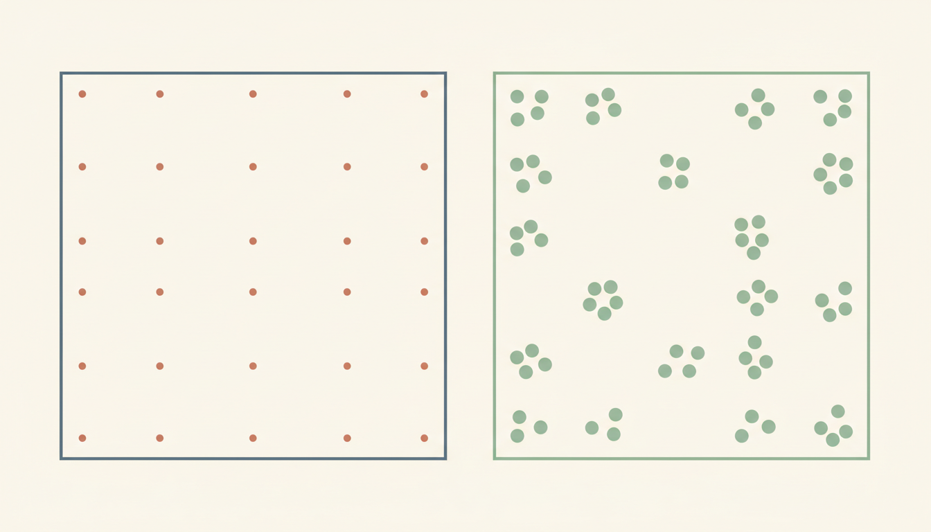
Equal headcounts do not guarantee equal precision. This original clustered-versus-independent survey example derives a design effect of 1.8 from a fully specified covariance model.
Chapter index
Audit the number of truly independent groups
Further worked tests: spending sample effort inside or across clusters
Chapters 1–4
1. Equal headcounts do not always carry equal information · 2. Declare the target and its variance model · 3. An explicit random-effects construction produces the covariance · 4. Derive the independent sample’s standard error
Chapters 5–8
5. Derive the clustered mean variance from covariance pairs · 6. Understand the design-effect formula and its limits · 7. Translate the design effect into an effective sample size · 8. Change cluster size while keeping n fixed
Chapters 9–12
9. What zero or negative ICC implies · 10. Study bias versus design variance · 11. Weights and stratification are additional questions · 12. An audit of standard errors and interval claims
Chapters 13–14
13. Frequently asked questions and exercises · 14. Connected subject reading and sources
Two hypothetical research teams each collect one hundred observations of the same continuous outcome. A reader may assume their sample means have identical statistical precision because the recorded headcounts agree. That conclusion is unsafe when one team samples individuals independently and the other samples people within shared clusters.
In Study I, all one hundred sampled values are independent under an explicit simple model. In Study C, the observations form twenty separate clusters with five people in each, and values within one cluster are positively correlated. Both studies have the same individual marginal variance of one hundred squared units.
Even when neither sample is systematically biased, the mean from the clustered observations can be more variable across hypothetical repeated studies. Members of the same cluster partly repeat shared information. Collecting five responses in the same household or classroom is not always statistically equivalent to taking five independent individuals from different contexts.
This article constructs a numerical covariance model and derives the exact variance inflation for the mean under those assumptions. The groups and outcomes are invented. The example teaches precision, not a claim about any actual school, household survey or trial.
Let Y be a continuous outcome measured in abstract units. Suppose the target mean is μ and every individual has marginal variance σ²=100 units squared, so the marginal standard deviation is ten units. For simplicity we consider unbiased sample means and ignore finite-population corrections in the worked model.
In Study I, one hundred observations are independent with the same mean μ and variance 100. The variance of their arithmetic mean is 100/100=1, and its standard error, assuming the variance is known, is one outcome unit. This is our reference.
Study C also observes exactly one hundred people, but the arrangement is twenty clusters of size five. Within each cluster any two distinct values have covariance twenty outcome units squared; observations from different clusters have zero covariance. Thus within-cluster correlation ρ=20/100=0.2.
The covariance assumptions are stipulated mathematical quantities, not estimates from real data. Their benefit is that every resulting number can be independently reproduced from variance-of-a-sum identities. A real complex survey may also need selection weights, stratification and multi-stage sampling factors.
One coherent way to generate clustered observations is Y_ij=μ+U_j+E_ij, where U_j is a cluster-level shared effect, and E_ij is a separate person-level deviation. Set Var(U_j)=20 and Var(E_ij)=80; assume all cluster effects are independent across j and all residual effects are mutually independent and independent of their cluster effect.
Then each observation has total variance 20+80=100. Two distinct people in the same cluster share U_j, so their covariance is twenty. People in different clusters have independent cluster effects and residuals, giving covariance zero. This construction exactly delivers the assumptions without a vague statement that classmates are ‘similar’.
The intracluster correlation coefficient, or ICC, is covariance between two distinct members of the same cluster divided by the marginal variance, here 20/100=0.2. Under this exchangeable model, every pair in a cluster has the same correlation.
A real data-generating process need not have this symmetric covariance structure. Correlations can differ across members, cluster sizes and outcomes. We use an exchangeable equal-size design because it makes the key information-loss mechanism easy to derive.
Write the independent sample mean as Ybar_I=(Y₁+…+Y₁₀₀)/100. For mutually independent observations, the variance of the sum equals the sum of variances, namely 100 observations times 100 units squared per observation.
Divide by the square of one hundred because the entire sum is divided by one hundred. Var(Ybar_I)=(100×100)/10000=1. Therefore SE(Ybar_I)=√1=1, in the original outcome units.
The standard error here quantifies repeated-sampling variation of the sample mean under the stipulated model and known variance. It is different from the standard deviation of individual outcomes, which is ten. Confusing individual variation with sampling precision introduces a factor of roughly √n.
An estimated standard error based on a real sample would include estimation uncertainty and appropriate design assumptions. Our numerical SE is a theoretical model consequence, used to compare two designs on equal footing.
Let Ybar_C be the average of all one hundred observations across twenty groups of five. When observations are correlated, Var(sum Y_i) includes not only the one hundred individual variances but also covariance terms between distinct pairs.
There are N=100 diagonal variance terms, each equal to 100. Within each of twenty clusters, five members each have four other members, giving 20×5×4=400 ordered within-cluster distinct pairs. Each corresponding covariance is twenty. Different clusters contribute no covariance under the model.
Thus Var(sum)=100×100+400×20=10000+8000=18000. Divide by N²=10000 for the arithmetic mean, yielding Var(Ybar_C)=1.8. Its standard error is √1.8≈1.341641 outcome units.
The two studies still have n=100 and individual standard deviation ten. Clustering has made the sampling variance eighty percent larger and the standard error roughly thirty-four percent larger. A count-only comparison would miss that difference.
For equal clusters of size m with common intracluster correlation ρ, the mean variance inflation relative to independent observations under the same marginal variance is D=1+(m−1)ρ. Here m=5 and ρ=0.2, so D=1+4×0.2=1.8.
Divide the clustered variance 1.8 by the independent variance one to obtain exactly that ratio. The design effect compares variances, not standard errors. The standard-error ratio is √D≈1.34164, not 1.8.
The CDC National Health and Nutrition Examination Survey variance tutorial explains design effects and the danger of standard software that ignores clustering. The cluster-trial design tutorial describes the equal-cluster formula and its assumptions.
This expression is not a universal correction for every survey. Unequal cluster sizes, sampling without replacement, weighting, stratification, outcome-dependent ICC and complex multi-stage design can change the right variance estimator. Use the model that reflects the actual collection mechanism.
A convenient rough comparison is n_eff=n/D, the size of an ideal independent sample that would produce the same mean variance under the same marginal variance. For Study C, n_eff=100/1.8≈55.56. This is an information-equivalent count, not a claim that only fifty-six people answered the survey.
The actual hundred people still matter, and their individual values can support other analyses. Effective sample size depends on the statistic and the assumed dependence. It is not an inherent permanent attribute of the data set regardless of the target variable.
Comparing n=100 independent with n=100 clustered should therefore not lead to identical confidence intervals based merely on the printed sample size. Under the toy model with known variance, the conventional normal-theory ±1.96 standard-error intervals would have half-widths about 1.96 and 2.63 outcome units, respectively.
Those numbers illustrate scale, not an automatically valid real-world confidence procedure. With only twenty clusters and unknown variance components, degrees-of-freedom and model-estimation choices matter. A real report should use a design-aware method rather than blindly applying a textbook normal approximation.
Imagine preserving one hundred measured people and the same within-cluster correlation ρ=0.2, but collecting ten clusters with ten individuals each. The equal-size design effect becomes 1+(10−1)×0.2=2.8. The theoretical variance of the sample mean becomes 2.8 instead of 1.8, and the standard error rises to √2.8≈1.6733 units.
The information-equivalent independent sample size falls to 100/2.8≈35.71. Enlarging each cluster while reducing the number of independent groups can reduce precision when values inside each cluster are similar. It may nevertheless save travel or setup costs; sampling choices balance statistics and field constraints.
At the other extreme, one hundred independent clusters of size one make the formula D=1 regardless of ICC, because there are no within-cluster pairs. This provides a consistency check rather than a recommendation to redefine arbitrary observations as independent without evidence.
The comparison assumes the same individual variance and pairwise ICC under both cluster arrangements, which is a model assumption. Real clusters can have unequal sizes, different means and changing dependence; those complications require separate investigation rather than careless substitution into a simple formula.
When ρ=0, the exchangeable model makes D=1+(m−1)×0=1. There is no extra covariance contribution to the sample mean variance. Group labels might still exist operationally, but under this narrow model they do not inflate this particular variance.
If within-cluster correlation is positive, D exceeds one and independence-based standard errors understate repeated-sampling uncertainty. The effect grows with m at fixed positive ρ, because each new person creates more correlated pairs within the group.
Negative within-cluster correlations are mathematically possible and could make D below one. For m=5 the exchangeable correlation matrix requires ρ≥−1/4 to remain positive semidefinite. A calculated ICC below that bound is incompatible with our simple equal-correlation five-member covariance model and signals a modelling or estimation problem.
The common classroom message that clustering always reduces precision is too broad. Positive within-group dependence often does so, but the result depends on the outcome, design and actual covariance structure. State the assumptions rather than substituting a convenient slogan for a variance calculation.
Study C’s sample mean can remain unbiased for μ under our equal-weight equal-cluster model. Its sampling variance is higher because people within each group share a random component. Unbiasedness and precision are distinct statistical properties.
If a convenience sample systematically excludes particular communities, both a large independent sample and a clustered sample can be biased regardless of their calculated standard errors. A tiny standard error does not correct a wrong sampling frame.
Likewise, the design effect formula does not magically repair nonresponse, incorrectly recorded outcomes or a poor estimator. It quantifies the variance ratio under the specified conditions. A report can need both a selection-bias audit and a cluster-aware variance method.
Compare the linked Stratified Samples, Population Weights and Misleading Means. That article changes the representation weights required for a population mean. Here the main issue is correlation among observations and the precision of an otherwise compatible mean estimator.
CHAPTER 11 OF 14
11. Weights, stratification and dependence are different design features
A real survey may oversample a small population group, select intact schools as clusters, and stratify primary sampling units across regions. Each feature answers a different design question. The estimator’s weights address unequal selection and adjustments; stratification and clustering affect variance estimation through different mechanisms.
A single unqualified ‘design effect of 1.8’ should not be copied across every variable. Correlation can be strong for a household consumption variable and weak for another outcome measured from the same respondents. Weight variation can also contribute its own precision costs or gains.
The CDC NHANES tutorial on variance estimation emphasises that weights and design variables need to be handled appropriately and that standard software ignoring complex sampling can produce misleading significance tests.
Our model has no unequal weights and all clusters are the same size. That choice isolates intracluster covariance so the effect is easy to see. Applying it to an actual multi-stage design without checking cluster identity, strata and sampling fractions would not meet the same analytical standard.
Begin by identifying the unit of observation and the unit of independent selection. One hundred survey responses collected from twenty selected classrooms do not have the same dependence structure as one hundred separately selected people scattered across a sampling frame.
Then report the actual number of clusters, respondents per cluster, whether sizes are equal, the outcome-specific ICC estimate if appropriate, weights, stratification and nonresponse. Document how uncertainty was calculated, including the type of standard error or replicate-weight method and any small-cluster correction.
A common software failure is to run a default standard-error routine that treats every row as independent simply because the file contains one row per respondent. Data-frame row count is not a proof of statistical independence. Correct analysis uses the selection design and covariance assumptions.
The CDC describes Taylor-series linearisation and replication methods for complex surveys. The right calculation may be more complicated than our one-line exchangeable design effect, especially for ratios, nonlinear estimators and subgroup analyses. A formula should be treated as a checkable model-specific result, not a universal shortcut.
Did the clustered study lose forty-four actual participants? No. Its data file still has one hundred distinct observations. The effective n≈55.56 is a precision comparison with an ideal independent sample for the specified mean and model, not a count of missing respondents.
Is ICC a type of bias? No. It measures within-group dependence relative to individual marginal variation in an exchangeable model. Positive ICC can inflate variance even when the estimator is unbiased.
Why not simply multiply the standard error by D? D is a variance ratio. Standard errors scale with its square root. Multiplying a standard error by 1.8 instead of √1.8 would confuse squared units with original units.
Can equal sample sizes ever have equal precision despite clustering? Yes. Under our model, ICC zero implies D=1. Design-based sampling and other complexities still need checking before claiming exact equality in a real study.
Practice: with m=4 and ρ=0.1, calculate D=1.3, and for n=120 calculate n_eff≈92.31. Then use m=8 and the same ρ to obtain D=1.7. Explain why adding more members to each group changes dependence even if the total headcount were held fixed.
Study I and Study C each have n=100, individual variance 100 and a compatible mean estimand. Study I’s mean variance equals one. Study C’s equals 1.8 under twenty clusters of size five with ICC=0.2. The increased standard error follows from the covariance terms, not arithmetic uncertainty about the responses.
Return to The Gold Standard of Statistics and Stratified Samples and Population Weights for the broader statistical reporting questions.
The authoritative CDC NHANES variance-estimation guide defines design effects and explains the risk of incorrect software uncertainty, while the cluster-trial design tutorial describes the equal-size ICC relationship and its scope. They are methodological sources; the invented cluster observations are not from those studies.
The practical standard is to preserve the sampling design rather than treating observations as a bag of independent spreadsheet rows. Continue through the Gold Standard hub and How X Works.
Advanced worked extension: covariance counting and design sensitivity
It is possible to verify the 1.8 design effect by two independent routes. The pair-counting method sums all individual variances and within-cluster covariances; the hierarchical random-effects method decomposes the sample mean into shared cluster effects and independent residual effects. Agreement of the two calculations is a useful internal quality check.
For twenty clusters each containing five responses, write Ybar=μ+(1/20)ΣU_j+(1/100)ΣE_ij. The shared-effect term has variance 20/20=1 because there are twenty independent cluster effects each of variance twenty. The residual term has variance 80/100=0.8. These add to 1.8. That matches the covariance-pair calculation without enumerating all four hundred ordered within-cluster pair terms.
Under a different decomposition with shared variance zero and residual variance one hundred, the sum-of-cluster-effects contribution vanishes and the variance returns to one. That is the independent case. Under shared variance forty and residual variance sixty, ICC becomes 0.4 and m=5 yields D=1+4×0.4=2.6, hence an SE ratio √2.6≈1.612 and effective n≈38.46.
Suppose an analyst had calculated a nominal mean of 50 outcome units. Under the known-variance idealisations, a simple ±1.96×SE normal half-width would be ±1.96 for the independent sample and ±2.630 for the clustered one. The centres may be equal but the precision differs. Those values are pedagogical normal-theory comparisons, not automatically valid confidence intervals from only twenty observed clusters when covariance parameters must be estimated.
The ICC must belong to the particular measurement being analysed. A survey of the same one hundred respondents might exhibit one dependence level for household income and a very different level for whether a respondent owns a bicycle. The design effect of an estimator is therefore variable- and design-specific; copying the 1.8 adjustment mechanically to every analysis would be unjustified.
For actual complex-sample analyses, record primary sampling units, strata and weights, then choose a design-aware variance method. The CDC guide describes why this is necessary. Our exercise offers a transparent diagnostic model so analysts recognise the dependence issue before selecting software.
Return to chapter index · Statistics subject root
| Statistic | Independent I | Clustered C |
|---|---|---|
| Recorded respondents | 100 | 100 |
| Groups and members | Independent | 20 × 5 |
| Individual variance | 100 | 100 |
| Within-group ICC | 0 | 0.2 |
| Mean variance | 1.0 | 1.8 |
| Standard error | 1.0000 | 1.3416 |
| Design effect | 1 | 1.8 |
| Effective n | 100 | 55.56 |
Further worked tests: spending sample effort inside or across clusters
Consider the same random-effects model Y_ij=μ+U_j+E_ij with shared cluster variance twenty and individual residual variance eighty. If there are c equally sized independent clusters of m respondents, the mean of all cm observations has variance Var(Ybar)=20/c+80/(cm). This expression separates the shared uncertainty, which averages over clusters, from individual residual uncertainty, which averages over all people.
With twenty clusters of five, the shared contribution is 20/20=1 and the residual contribution is 80/100=0.8, giving total variance 1.8 as calculated earlier. It is helpful to see that the design effect is not an unexplained multiplier: it follows from how independent cluster effects and person-level residuals enter the mean.
Suppose a researcher interviews five more people inside each of the same twenty clusters. The sample grows to two hundred observations with m=10. The shared contribution remains 20/20=1 because the number of independent groups has not increased. The residual contribution becomes 80/200=0.4, so mean variance falls only to 1.4. More observations help, but some uncertainty persists at the cluster level.
Instead, suppose the researcher samples twenty additional independent clusters of five, reaching forty clusters and the same two hundred people. The shared part is now 20/40=0.5, and the individual part remains 80/200=0.4. Total variance is 0.9. Under the stipulated equal-cost statistical model, spreading responses across more independent clusters gives more precision than simply increasing the take within already selected groups.
These are theoretical comparisons rather than sampling-plan recommendations. In actual fieldwork, reaching a new location or school may cost much more than taking extra observations within one site. Optimal design therefore balances precision with operational cost, access, nonresponse, safety and the target outcomes.
At the original m=5, reducing ICC from 0.2 to 0.05 changes the simple design effect to 1+4×0.05=1.2. The corresponding effective sample size for one hundred people becomes about 83.33. Raising ICC to 0.5 makes design effect 3.0 and effective n roughly 33.33. The recorded headcount never changes in either comparison.
ICC itself should not be treated as a fixed property of a neighbourhood or class independent of the outcome. One variable can have strong household similarity while another has little. A meaningful precision report ties the intracluster correlation estimate to the variable, population and analysis actually performed.
To validate software output, compare its estimated mean variance with a transparent hand calculation where possible. If a default procedure returns independent-observation standard errors in a clustered study, check whether it was told which sampling units are shared. The CDC survey variance tutorial explains why complex-sampling attributes matter to confidence limits and significance testing.
Return to chapter index · Gold Standard hub
Audit the number of truly independent groups
An effective sample size is often tempting to treat as a replacement for the original sample description. It should instead be presented alongside the actual number of people and clusters. A value such as n_eff≈55.56 describes the variance-equivalent precision of one estimator under our particular model. It does not reveal which respondents were selected or whether the sampled groups represent the target population.
When there are only a handful of clusters, estimating uncertainty can be more delicate than plugging an ICC into D=1+(m−1)ρ. Large-sample normal approximations may be weak, and estimators that use cluster-robust covariance matrices can require small-sample corrections or different degrees-of-freedom choices. A well-documented analysis states the inferential method rather than merely printing a design effect.
An instructive sensitivity report can compare several plausible ICC values before data collection. If a planned estimate depends strongly on whether ICC is 0.05, 0.20 or 0.50, the research team should recognise that the design has a meaningful dependence uncertainty. A pilot study or appropriate previous evidence may help to choose a realistic range; the worked figures here are invented.
Finally consider what happens when some selected clusters do not participate. Missing entire groups can create representation problems in addition to reducing precision. Increasing the number of individual respondents within the remaining groups is not always a substitute for replacing lost coverage across geographic or institutional strata. The sampling frame and dependence structure both require separate audits.