
Archaeological Diatom Analysis studies fossil silica structures from aquatic microalgae to investigate past wetlands, waterfronts, salinity and sediment formation. A 50% share of marine-affiliated valves does not mean the sea stood 50% higher. Correct interpretation begins with identification, context, counting convention and sediment history.
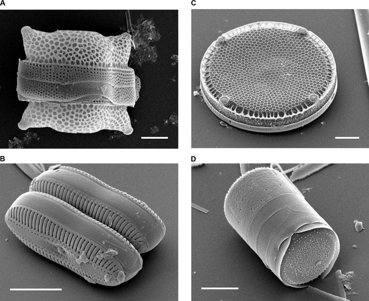
Our fictitious Harbour Marsh count changes from 20% marine-affiliated valves in lower H1 to 50% in upper H2. The exercise illustrates a relative composition, not a measured sea-level change or historical tsunami. The featured scanning electron microscopy images, courtesy Mary Ann Tiffany, are modern references and not specimens from this imagined excavation.
The Historic England 2025 Environmental Archaeology guide, Diatoms of North America and UCL Roman foreshore study provide method and real context. The eduKate Gold Standard requires direct answers, detailed worked evidence and independent transfer.


Find the diatom research question
Follow the full fictional core investigation, or use the five reading routes for the appropriate method.
Chapter index
Microfossils and habitats · Chapters 1–3
Taxonomic and sampling sources · Chapters 4–6
Counts and taphonomy · Chapters 7–10
Flooding, tides and ecology · Chapters 11–14
Reporting and transfer · Chapters 15–16
1. Diatom valves do not measure sea level directly
A fictional archaeological site called Harbour Marsh contains two sediment samples with different marine-affiliated diatom proportions. Diatom analysis studies fossil silica structures from microalgae that may reveal aquatic conditions, but an assemblage percentage is not the elevation of the sea. More marine-affiliated valves could reflect lasting salinity, short-lived marine transport, reworking or preservation changes.
The UCL Roman Thames foreshore diatom study offers a real example of using identifiable taxa and archaeological context to investigate tidal environments. Our imaginary counts are unrelated to its results. First ask what was recovered, then what historical explanation the evidence could test.
Back to chapter index · Next chapter
2. How diatom frustules preserve evidence
A diatom has a siliceous external cell wall, or frustule, typically comprising two valves and girdle bands. Sediments may contain complete structures, separated valves or fragments. These are not automatically separate original organisms. A fossil census must define its observed and counted units.
Use the modern electron micrographs courtesy Mary Ann Tiffany to distinguish valve, girdle bands and the shape of particular frustules. Diatoms of North America explains the anatomy. Ask whether one photographed broken edge can justify an intact-cell count; it cannot without a declared analytical convention.
Back to chapter index · Next chapter
3. Centric and pennate forms are not salinity categories
Diatom morphology is diverse; centric and pennate are broad structural groupings, not simple synonyms for marine and freshwater habitats. Ecology depends on taxa, life habit, and environmental tolerances. Many taxa are planktonic, attached to plants or living on sediments; their dead remains can then be transported.
Students inspect labelled source images and describe the geometry before researching each taxon’s ecological preference. A centric shape alone does not prove salty water. The lesson separates morphology from environmental diagnosis so that familiar-looking grains do not become unsupported stories about a shoreline.
Back to chapter index · Next chapter
4. Ecological preferences need suitable modern references
Salinity, acidity, oxygen, nutrients, current, substrate and other variables influence living diatom distributions. A fossil species’ modern ecological range can inform interpretation, but environmental preferences overlap and sometimes respond to multiple variables. A label such as ‘brackish-affiliated’ conveys a tendency, not universal exclusivity.
Give learners two modern ecology records for the same species from different environments. They should identify the overlapping tolerances before assigning it to a fossil assemblage. The archaeological diatom review discusses salinity and tidal applications while acknowledging taxonomic complexity.
Back to chapter index · Next chapter
5. Site context is part of the sample
Mud from a foreshore, lake bed, peat lens, tidal ditch or transported sand has distinct formation histories. Field records must preserve site, depth, sediment description, sample interval, structure, position and possible disturbances. A microscopically accurate identification cannot recover lost excavation provenance.
In the invented profile, H1 is coherent mud and H2 is coarse sandy sediment. Ask which sedimentary processes could account for the different matrix, and whether the samples are from equivalent depositional environments. The Historic England 2025 environmental guidance emphasises sampling plans tied to research questions.
Back to chapter index · Next chapter
6. Microscopy and safe sample processing
Diatom preparation isolates silica structures from sediments, commonly through specialist chemical processing and controlled microscopy. Handling, reagents, slide mounting, optics and analyst criteria can affect which remains survive and can be identified. These methods require qualified laboratory work rather than an unsupervised classroom procedure.
Students compare a complete analytical record with an attractive microscope image missing magnification, sample ID and processing history. They identify what the image can and cannot support. Use licensed images and prepared counts for school experiments; a demonstration of classification principles does not require chemical processing of archaeological deposits.
Back to chapter index · Next chapter
7. Identify taxa only as far as the material permits
Species-level diatom identifications require recognisable diagnostic characters, suitable modern references and preservation adequate for inspection. Partly dissolved valves can be recorded at genus or broader group, or left indeterminate. Species concepts and nomenclature can change, so the reference used should be recorded.
Pupils classify a fictional complete valve and a damaged one. They justify why one supports a narrower identification. When a taxonomic key is updated, the original documented observation should remain so later readers can reassess the ecological interpretation without inventing features absent from the fossil.
Back to chapter index · Next chapter
8. Valves, fragments and denominator conventions
A percentage depends on which remains an analyst counts and how broken forms are treated. The two fictional Harbour Marsh samples each contain 200 identifiable valves under one mutually exclusive counting rule. Additional fragments are documented separately. Counting fragments as whole valves would change percentages without changing the original organisms.
Students recompute a marine-affiliated share when forty unclassified fragments are added to the denominator. They must say that the 50% becomes about 41.7% under this different rule, and that the two results do not answer precisely the same analytical question.
Back to chapter index · Next chapter
9. Calculating the freshwater, brackish and marine groups
Lower H1 has 80 freshwater-, 80 brackish- and 40 marine-affiliated valves. Upper H2 has 30, 70 and 100. Marine share rises from 20% to 50% within the declared count, while freshwater share falls from 40% to 15%. Neither statistic measures a change in metres of sea level.
The class writes an accurate table caption stating count categories, totals and the fictional context. A misleading caption would claim a marine transgression of a precise vertical height or an exact historic catastrophe. Students should identify the missing survey elevation, source ecology, independent age and sedimentological evidence needed for those claims.
Back to chapter index · Next chapter
10. Differential preservation and missing taxa
Diatom silica can dissolve or fragment in some sediments, sometimes preferentially damaging fragile forms. An apparent community shift could therefore reflect taphonomic loss as well as environmental change. A low total of identifiable valves may prevent a confident reconstruction at all.
The Horseshoe Lake study near Cahokia considers dissolution and low diatom intervals when interpreting ecological history. Pupils compare fictional preservation scores and ask whether raw percentages in damaged and intact samples can carry equal inferential weight.
Back to chapter index · Next chapter
11. Transport and reworked diatom shells
Diatoms recovered in an archaeological layer did not necessarily live there. Tidal water, floods, reworked shoreline sediment and human disturbance can introduce frustules from other habitats or times. A marine-affiliated assemblage in a ditch may reflect water movement rather than a permanent marine inlet.
Students sketch two alternatives for imaginary H2: persistent brackish conditions versus one sandy flood deposit transporting marine material. Grain size, erosional contacts, valve wear and additional cores could help distinguish them. The microscope alone cannot answer the formation question.
Back to chapter index · Next chapter
12. Tsunami, tide and storm claims need more than marine diatoms
Marine-affiliated valves may appear in sediments laid down during tsunamis, storm surges, tidal flooding or reworking. A single marine-rich interval is not a unique hazard signature. Independent sedimentology, event history and dating are required before naming a specific flood mechanism.
A study of Japanese coastal lakes investigated diatom patterns in historically attributed tsunami and typhoon deposits. Students should examine why its real analytical context differs from our hypothetical 200-valve table. A good conclusion proposes a hazard test, not a dramatic invented event.
Back to chapter index · Next chapter
13. Former sea level needs datum, elevation and chronology
Diatoms can contribute to reconstructions of freshwater, tidal or marine influence, but absolute or relative sea-level change also requires reference elevations, tidal ecology, compaction and dated sediment sequences. The observed thickness of an ash or sand layer is not itself sea-level change.
The UCL Pudding Lane report investigated a Roman foreshore near the tidal head of the Thames. Students identify the richer source controls that make its interpretation possible and explain why Harbour Marsh, with no surveyed site elevation or age model, cannot yield a reliable sea-level curve.
Back to chapter index · Next chapter
14. Aquatic habitat changes may have several causes
Diatom communities respond to nutrients, water movement, plants, sediment sources and climate. A shift from planktonic to attached forms could accompany eutrophication, changes in aquatic plants, depth or river inflow. Human activities might contribute, but diatom data do not directly count people or state agricultural decisions.
The Horseshoe Lake research explores diatom ecology around Cahokia with broader historical evidence. Give pupils two explanations for a hypothetical nutrient shift and ask what land-use chronology or sediment chemistry could distinguish them. Avoid equating ecological correlation with one person’s action.
Back to chapter index · Next chapter
15. Build an auditable diagram
A defensible diatom diagram preserves source taxon list, valve counts, denominator, treatment of fragments, sampling depths, preservation, preparation method, habitat classifications and chronology where available. Colour alone can mask those decisions, and a small labelled percentage without its source cannot be independently checked.
Students repair a fictitious infographic reading ‘50% seawater’ by adding actual valve categories, numerical sample totals and uncertainty. Ask whether a second researcher could recompute the data and identify the reference ecological preferences. If not, the chart may be attractive but is not a robust archaeological argument.
Back to chapter index · Next chapter
16. Transfer to an independent coastal sediment case
A new fictitious ditch has a dated-looking artefact, an undated sandy lens, broken marine-affiliated valves and an intact freshwater horizon beneath. Students calculate what the fossil counts show, consider whether the valves were reworked and identify what the artefact can legitimately date.
An excellent answer makes two competing formation hypotheses and proposes field and laboratory evidence to choose between them. It does not declare a tsunami, stable shoreline or date of human occupation merely because the biological microremains point towards marine transport. This is the transferable gold-standard method.
Worked two-sample valve count
| Fictional class | H1 | H2 |
|---|---|---|
| Freshwater-affiliated | 80 / 200 = 40% | 30 / 200 = 15% |
| Brackish-affiliated | 80 / 200 = 40% | 70 / 200 = 35% |
| Marine-affiliated | 40 / 200 = 20% | 100 / 200 = 50% |
| Classified valves | 200 = 100% | 200 = 100% |
The table describes recovered fossil composition. It does not identify one hazard, elevation or year. The fictional source has no independently dated age model, and the taxonomic categories are simplified for instruction.
Case study: two layers are not two sea-level measurements
The base classroom table is H1: 80 freshwater, 80 brackish, 40 marine; H2: 30 freshwater, 70 brackish, 100 marine; both totals 200. The marine percentage increases by 30 percentage points. That is a proportion of counted valves and cannot be transformed into 30% of the surrounding landscape, a metre elevation or a calibrated year without new measurements.
Pupils identify the missing information, then design a field visit plan on paper: map exact sampling locations, examine contacts, obtain appropriate elevations and seek independent dating. Each proposed observation should connect to one of the claims currently unsupported. The objective is to move from valid arithmetic to a testable water-history investigation.
Case study: a broken shell can create a false abundance
In a second imaginary H2 count, twenty damaged diatom frustules split into multiple fragments. An analyst who counts fragments as independent intact organisms can inflate a taxon disproportionately. Students are asked to preserve complete-valve counts and broken pieces separately, then explain which denominator a plotted ecological percentage should use.
The strongest answer recognises why the same specimen may appear in a preservation tally and in an identification record but should not automatically count twice as an original cell. A transparent method is more useful than a deceptively exact result based on an unreported convention.
Case study: a real Thames waterfront is not the invented harbour
Battarbee’s Roman Pudding Lane study identified many diatom taxa in the foreshore near early Roman quay structures. It used their ecological associations to investigate a complex tidal setting. The real result does not date or locate imaginary Harbour Marsh.
Students compare source quality: the real study records taxa and context; the teaching model has only three ecological groups. They should articulate the legitimate transfer—a method for interpreting water environments—without copying numerical findings, locations or dates from an unrelated archaeological record.
Case study: an isolated storm pulse
A fictional sandy lens has several marine-associated forms and an erosional lower boundary. One interpretation is a short-lived flood bringing sediment inland; another is continuous brackish water with changing energy. A convincing distinction would require sedimentology, age control and ecological comparisons rather than a vote on which story sounds more exciting.
Students write an evidence table listing support, counterevidence and next tests for both models. A good answer may leave the origin unsettled. The skill is not proving that no tsunami ever happened; it is knowing when a single fossil assemblage cannot identify one.
Case study: low preservation defeats an attractive graph
A later imaginary sample contains only five identifiable valves among abundant corroded fragments. Its calculated percentages may look extreme because the denominator is tiny and biased. Pupils must decide whether the result should be published as a confident environmental reconstruction or as a very limited observation.
They should report the five valves and preservation issue honestly, then propose other adjacent levels or comparative environmental evidence. An interval with weak source quality can still inform sampling strategy, but it cannot be used as a strong climatic or coastal history on its own.
Case study: communicating findings to a visitor
Students draft a 100-word museum sign describing evidence for changing aquatic conditions at fictional Harbour Marsh. It must identify which diatom assemblage was counted, why source transport remains possible and what independent data are needed before stating a cause or date.
A sign explaining that marine-associated valves become more common is scientifically clearer than one announcing an undated coastal catastrophe. This is not timid writing; it is accurate public communication rooted in traceable archaeological evidence.
Four-lesson learning sequence
- Lesson 1: identify frustules, valves and ecological source descriptions with appropriate microscopy captions.
- Lesson 2: inspect invented contexts, fragility, transport and the valve-count denominator.
- Lesson 3: calculate and discuss marine-affiliated proportions without claiming a measured shoreline elevation.
- Lesson 4: evaluate a new mixed sediment sequence and write a source-aware public summary.
Advanced ecological calibration: freshwater is not a single universal label
In a fictional teaching reference, Taxon A is commonly associated with freshwater but tolerates a broad range of conductivity, while Taxon B has a narrower salinity tolerance. If the fossil assemblage contains A but not B, the analyst cannot automatically infer exact salinity, because both taxa respond to multiple factors and the absence of B could reflect preservation or sampling. Students should distinguish modern observed tolerance from a fixed diagnostic threshold. A reliable ecological assignment needs source location, environmental measurements, taxonomic quality and modern comparison material appropriate to the historical region.
Next provide a series of hypothetical modern reference samples collected along a coastal salinity gradient, with each sample listing conductivity, pH and identified valves. The learners propose what a formal transfer-function study would require before converting ancient assemblages to environmental estimates. They must recognise that even a statistically fitted model has uncertainty, potential poor analogues and a geographically restricted training set. A three-colour classroom diagram is not a substitute for those controls. This gives students a precise definition of what additional evidence would make a quantitative water-history reconstruction legitimate.
Advanced field case: valves may travel while a sediment bed remains local
Imagine the fictional Harbour Marsh H2 sand layer receives river water carrying old marine sediment from an eroding coastal bank. Under this model, the marine-affiliated valves in H2 could predate the final formation of the sand layer and represent transport rather than an episode of saltwater habitat at the excavation. Another model proposes direct saline inundation. Both could yield superficially similar diatom proportions. Students should examine sediment grading, erosional boundaries, valve breakage and possible source exposure rather than use the percentage alone.
Ask pupils to build a source-route diagram showing where the valves lived, how they moved and when the measured archaeological layer accumulated. They should record each event separately. If a date from a twig is recovered within the sand, it may help with deposition chronology under suitable association but does not automatically date the original growth of every fossil valve. This teaches that biological source, particle transport and final burial are three distinct historical steps.
Advanced preservation case: an interpretable sample is not necessarily the largest count
A fictional lower core sample has 220 valve fragments but only twenty confidently identifiable complete or diagnostic valves. Another has 120 well-preserved identifiable valves. The first sample contains more siliceous pieces in total, yet its ecological signal may be weaker. Pupils should decide how to report both totals and which can enter the defined species-proportion sum. They must not declare a high-confidence environmental transition solely because the microscope field contains many particles.
Now change the preservation profile so fragile freshwater taxa are disproportionately broken while sturdy marine-affiliated valves survive. The apparent marine share could rise without a matching increase in original marine input. A valid interpretation requires assessing taxon-specific preservation and sample preparation. An unambiguous ‘not enough reliable data’ result may be more informative than a confident plot that mistakes dissolution and breakage for a change in the living waterbody. Encourage pupils to communicate the limitation explicitly, not hide a sample because it complicates the figure.
Advanced historic-waterfront case: settlement use and aquatic ecology differ
The genuine Roman Thames study at Pudding Lane investigated deposits associated with a waterfront structure, but the diatom assemblage does not identify individual harbour workers, exact vessel traffic or one economic purpose by itself. The biological evidence helps reconstruct the depositional aquatic environment; the cultural interpretation relies on the quay structure, site stratigraphy and other archaeological materials. Our fictional Harbour Marsh has no equivalent securely documented waterfront architecture.
Students receive two fictional maps: one marks a possible timber structure and the other shows the diatom core position. Ask whether the core can be treated as direct evidence for the structure’s construction year or trading intensity. It cannot. A later historically dated timber could constrain part of the settlement history under suitable association, while diatoms might illuminate water conditions nearby. Strong historical writing reports those contributions separately before proposing a combined narrative. This prevents diatom analysis from absorbing the work assigned to Chronology or Historical Cartography.
Advanced hazard case: the marine signal is real but the event name is not
Suppose a coastal storm leaves a sandy layer rich in marine diatoms, while a tsunami can produce another marine-rich sand layer in a comparable environment. The same biological observation may be consistent with both. A responsible hazard attribution needs coastal topography, grain size, inland reach, sedimentary structures, chronological comparison with historical events and an understanding of local storm and tsunami processes. Marine-affiliated taxa alone do not make a unique fingerprint for either event.
Give students two published source summaries—one concerning the Japanese coastal-lake comparison and another describing Harbour Marsh’s invented counts. They identify which observations belong to the real study and which are not available in the teaching example. The final short response should avoid phrases such as ‘the diatoms prove a catastrophic tsunami’ until external evidence warrants them. Pupils learn how to keep a hypothesis useful without misrepresenting its certainty.
Advanced report audit: six fields needed for independent reuse
An archaeological diatom report should let another researcher identify the exact sediment source, sampled interval, preparation history, classification references, count denominator, preservation and calibrated chronology when present. Add measured elevations or water-chemistry comparisons only when an actual survey or model supports them. An isolated 50% label may be a true mathematical output under one scheme, but is not a reproducible environmental history. The archive must preserve the raw observations that produced it.
Ask one group to write the fictional H2 result and another group to recompute it without seeing the original worksheet. If they lack the 100-marine-of-200-valves raw data or fragment inclusion rule, they cannot check the figure. Have students add the missing fields, including a note that ecological grouping was illustrative and that the deposit may be transported. Then ask for a visitor-facing summary of one or two sentences that retains this provenance without overwhelming the reader. Good research supports both technical verification and clear public explanation.
A source-specific assessment rubric
| Stage | What full-credit work shows | Unsupported shortcut |
|---|---|---|
| Microscopy | Identifiable valves, taxonomic reference and preservation | Assigning habitat from centric/pennate shape alone |
| Count | Original numerator, denominator and treatment of fragments | Calling a valve share the percentage of sea water |
| Context | Source horizon, formation and potential sediment reworking | Equating marine input with sustained local habitat |
| Time and place | Independent age control and surveyed context as necessary | Inventing an exact sea level or tsunami date |
| Transfer | Testing a new core with an alternative formation model | Repeating the original answer irrespective of evidence |
After marking the fictional Harbour Marsh answers, introduce a new sediment layer with a modern drainage feature cutting through it. Learners should revise only the inferences affected by the newly revealed disturbance. An adaptable, transparently qualified conclusion demonstrates that the method has been understood beyond one worked example.
Frequently asked questions
Does 50% marine-affiliated diatoms mean half the ground was seawater?
No. It means half the defined counted valves belonged to a chosen ecological category.
Can a marine valve prove a tsunami?
No. Flooding, tides, storms and reworking require independent discrimination.
Are all centric diatoms marine?
No. Shape and habitat are distinct variables.
Why preserve raw counts and fragment descriptions?
They allow another researcher to evaluate percentages and taphonomic biases.
Research and related eduKate guides
- Historic England Environmental Archaeology (2025)
- Diatoms of North America Frustule Glossary
- UCL Roman Pudding Lane Diatom Report
- Archaeological Diatom Analysis Review
- Horseshoe Lake and Cahokia Research
- Coastal Tsunami and Typhoon Diatom Research
- Mary Ann Tiffany Micrographs, CC BY 2.5
- Teaching Palynology
- Teaching Geoarchaeology
- The Gold Standard hub
The gold standard is an independently defensible description of fossil diatom valves and their depositional context, followed by a cautious water-history interpretation another reader can check.
Place diatom evidence alongside other microfossil groups, recovery methods and chronological interpretation in The Gold Standard of Micropalaeontology.