
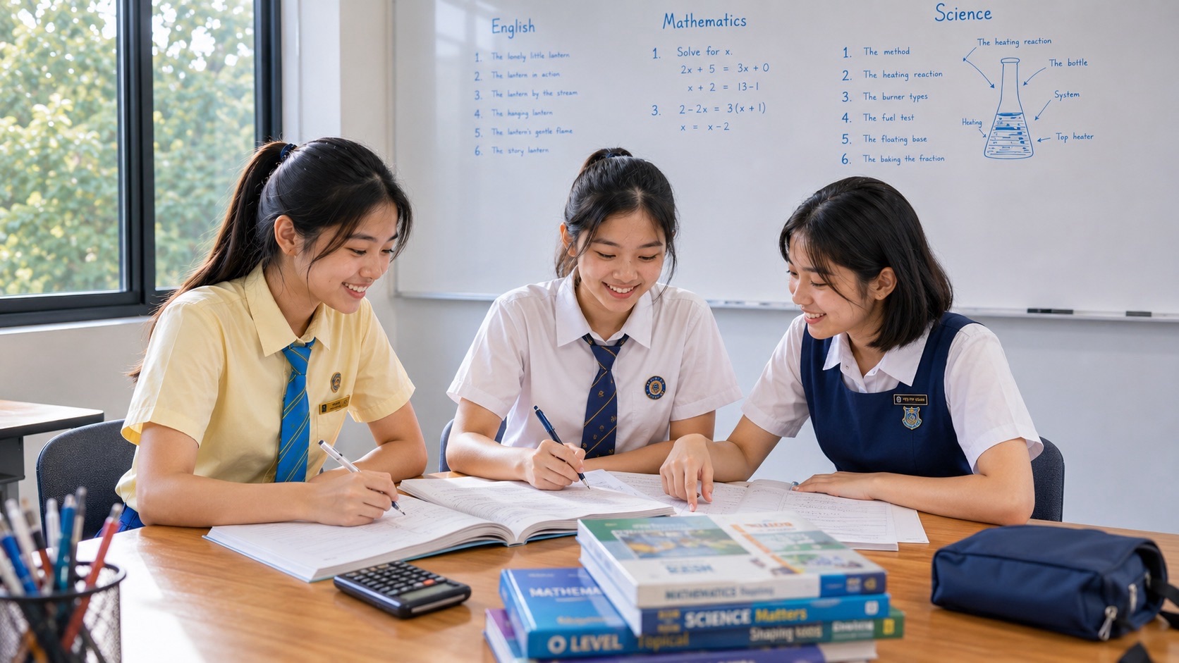
Secondary 2 G2 Mathematics includes interpreting dot diagrams, histograms and stem-and-leaf diagrams, recognising misleading statistical displays, choosing mean, median or mode, calculating an estimated mean for grouped data, and finding the probability of a single event. These are the MOE Secondary Two G2 topics in Statistics and Probability. The school’s Secondary 2 tests assess this learning; SEC Mathematics K210 is the later national qualification.
For parents, the goal is to teach a child to ask what the data mean before doing the arithmetic. A perfectly calculated average may still misrepresent a group if one observation is unusual. A beautifully drawn graph can mislead if the axes or intervals are unclear. This guide provides a step-by-step sequence, complete miniature data sets and ways to check understanding without creating unnecessary tuition pressure.
- Dot diagram: each dot should represent an observation, organised along a scale.
- Stem-and-leaf: retain individual values and supply a clear key.
- Histogram: show frequency across numerical intervals with adjacent bars.
- Central tendency: know when to use mean, median or mode and how an outlier matters.
- Grouped mean: use class midpoints as estimates when exact raw data are unavailable.
- Probability: list equally likely outcomes for one chance event and state assumptions.
1. Start with a genuine question about a small data set
Eight pupils record the following number of minutes needed to complete a small task: 12, 14, 14, 17, 21, 22, 27, 31. The question is not ‘Which formula should I use first?’ Ask instead: What are we measuring? How many pupils were involved? Are the data already in ascending order? Which comparisons are fair?
The range of this small collection is 31 − 12 = 19 minutes. Its median is the mean of the fourth and fifth values because there are eight observations: (17 + 21)/2 = 19 minutes. The mode is 14 minutes because that value occurs twice, more than any other. The total is 158 minutes, so the mean is 158/8 = 19.75 minutes. These three measures answer different questions.
| Measure | Value | Meaning and limitation |
|---|---|---|
| Mean | 19.75 minutes | Uses all eight numbers; changes when an unusually large or small value changes |
| Median | 19 minutes | Middle position after ordering; resists an unusually large observation better |
| Mode | 14 minutes | Most frequently occurring value in this collection; there may be no mode or multiple modes |
| Range | 19 minutes | Simple spread between maximum and minimum, not itself a measure of central tendency |
2. What a dot diagram shows
A dot diagram places individual observations above their value on a number line. For the collection 2, 2, 3, 5, 5, 5, 6, there would be two dots above 2, one above 3, three above 5 and one above 6. There are seven dots altogether. Without even calculating an average, a student can see that 5 is the most common value.
Parents can make this visible with coins on a sheet of squared paper. Label the number line before stacking coins. Then ask the child to reconstruct the original observations from the dots. If they cannot reconstruct the raw list, they may be reading the display as an illustration rather than a representation of individual measurements.
3. How a stem-and-leaf diagram keeps the actual observations
Use the eight task times again. Make the tens digit the stem and the ones digit the leaf, keeping leaves sorted. The display is 1 | 2 4 4 7, 2 | 1 2 7, 3 | 1. State the key: 1 | 2 means 12 minutes. The key is essential because a different context might use decimals.
| Stem (tens) | Leaves (ones) | Values shown |
|---|---|---|
| 1 | 2 4 4 7 | 12, 14, 14, 17 |
| 2 | 1 2 7 | 21, 22, 27 |
| 3 | 1 | 31 |
The total number of leaves is eight; this must match the number of raw values. Sorting within each stem allows the median and mode to be found without losing information. A histogram, by comparison, organises values into intervals and typically no longer shows their individual exact values.
4. What makes a histogram different from a bar chart
A histogram displays frequencies in numerical intervals, such as 0–9 minutes, 10–19 minutes and 20–29 minutes. Those intervals are adjoining parts of a numerical scale; accordingly their bars touch. A bar chart of unrelated categories such as English, Mathematics and Science uses separate categorical bars.
For example, a school collects the times for eight students and groups the results as 0–9 minutes: 2 students; 10–19 minutes: 4 students; 20–29 minutes: 2 students. With equal-width intervals, the bar heights can follow the frequencies 2, 4 and 2. Always state the interval boundaries clearly; if a school introduces unequal interval widths, do not assume that raw frequency is always the correct comparative height.
| Time class | Frequency | Midpoint for grouped-mean estimate |
|---|---|---|
| 0–9 min | 2 | 4.5 |
| 10–19 min | 4 | 14.5 |
| 20–29 min | 2 | 24.5 |
| Total | 8 | — |
5. The grouped-data mean is an estimate, not an exact reconstruction
When data are supplied only as grouped frequencies, one conventional estimate assumes observations in each class are represented by its midpoint. Using the table: 2 × 4.5 + 4 × 14.5 + 2 × 24.5 = 9 + 58 + 49 = 116. Divide by eight observations to obtain an estimated mean of 14.5 minutes.
The estimate cannot tell us exactly which times individual students recorded. For example, 10 and 19 both lie in the same class, yet the midpoint 14.5 substitutes for either in the grouped calculation. Explain that this is an estimate made with grouped data; do not assert that the true mean must equal 14.5.
6. Why the same graph can tell different stories
Suppose a chart compares scores of 72 and 75 and displays a vertical axis beginning at 70 rather than zero. The three-point difference may look enormous because the visible bars start near the plotted values. Sometimes a shortened axis is useful for showing a small variation, but it can mislead if viewers assume the bar lengths represent full magnitude.
Ask the child to inspect the title, sample size, units, scale, category boundaries and what has been omitted. A mathematically critical reader does not assume every chart is dishonest; they distinguish a helpful design choice from one that hides meaningful context.
7. Mean, median and mode: why ‘average’ needs interpretation
Imagine five waiting times: 2, 3, 3, 4 and 30 minutes. The mean is 42/5 = 8.4 minutes, the median is 3 and the mode is 3. The 30-minute observation is unusual compared with the others. If a parent asks how long the wait usually is for four of the five visits, the median may offer more helpful context than the mean.
That does not make the mean wrong. For planning the total waiting time across repeated visits, the mean can be valuable. The choice of summary depends on the question. Explain that a statistical measure is a tool for a purpose, not the answer to every possible interpretation.
8. Probability is a measure of chance, not a promise
Suppose a bag holds three identical red counters, two identical blue counters and five identical green counters, mixed and drawn fairly. There are ten equally likely counters. The probability of red in one draw is 3/10; the probability of not red is 7/10. The two probabilities add to 1.
A 3/10 probability does not mean exactly three of the next ten draws must be red. Chance events can vary in short sequences. The simple equally likely formula also relies on the assumption that every individual counter has an equal chance of selection. State the model before dividing.
9. One roll of a fair die: list the sample space
The possible results of one roll of a fair six-sided die are {1, 2, 3, 4, 5, 6}. The event ‘roll an even number’ has favourable outcomes {2, 4, 6}; the probability is 3/6 = 1/2. The event ‘roll a number greater than 4’ has {5, 6}; its probability is 2/6 = 1/3.
A student may count ‘6’ but forget that 5 is also greater than 4. The best repair is to list the outcomes clearly. Avoid jumping prematurely into multi-stage tree diagrams: the Secondary 2 G2 list specifies probabilities of single events and listing simple outcome spaces.
10. Eleven concept checks for the parent
| Check | Question | Answer or expected reasoning |
|---|---|---|
| 1 | Data 2, 2, 3, 5, 5, 5, 6: how many observations? | 7 |
| 2 | In that set, what is the mode? | 5 |
| 3 | Does a stem-and-leaf need a key? | Yes; a key explains the place value |
| 4 | Is 1 | 4 always 14? | No; the key and measurement units govern the meaning |
| 5 | Why do conventional histogram bars touch? | The numerical class intervals are adjoining |
| 6 | Can grouped frequencies alone recover every exact value? | No |
| 7 | What midpoint represents 10–19? | 14.5 |
| 8 | What is the grouped-mean estimate for frequencies 2, 4, 2 in classes 0–9, 10–19, 20–29? | 14.5 |
| 9 | What is the median of 2, 3, 3, 4, 30? | 3 |
| 10 | Fair die: probability of an even number? | 1/2 |
| 11 | Bag with 3 red of 10 equal counters: probability of not red? | 7/10 |
11. How to diagnose the first wrong step
| Observed mistake | Conceptual issue | Useful next activity |
|---|---|---|
| Leaves are not sorted; median wrong | Order and representation are unstable | Rebuild stem-and-leaf from an ordered list |
| Grouped mean claimed to be exact | Approximation is not understood | Invent two different raw data sets with the same class frequencies |
| Median calculated without sorting | Positions in a data set are unclear | Put number cards in order before finding the centre |
| Histogram treated like labelled categories | Numerical intervals vs categories confused | Place each observation in its numeric class |
| Graph axis deliberately cropped without noticing | Scale interpretation absent | Redraw using zero baseline and compare appearance |
| Chance of red reported as 3 instead of 3/10 | Outcomes not related to total | Write favourable/total before computing |
12. A seven-day Statistics and Probability practice plan
- Day 1: gather a tiny anonymous set of numbers, such as numbers of pages read by five fictitious students, and explain the measurement.
- Day 2: draw a dot diagram and reconstruct the values from it.
- Day 3: draw a stem-and-leaf diagram with a clear key; locate median and mode.
- Day 4: group an example set into sensible equal-width intervals and sketch a histogram.
- Day 5: find an estimated mean from grouped data and explain why it is approximate.
- Day 6: list the outcomes for one fair die roll or one counter draw; calculate simple event probabilities.
- Day 7: interpret one misleading graph and redo mistakes from earlier days.
A family can spread this work over more than a week. There is no benefit in turning every evening into another test, especially when other school subjects and CCA commitments are demanding. A patient explanation about what a graph represents is often more valuable than a large number of calculations.
13. Why this matters outside Mathematics
Science classes require pupils to understand tables, graphs, averages and uncertainty. Geography and the Humanities often present numerical evidence in charts. Everyday news and product claims use percentages and probability language. Students who habitually inspect sample size, axis scale and assumptions are developing habits useful beyond one examination.
The topic can therefore motivate a child who sees Mathematics as only rules and sums. Show an accessible data question that matters to the student, but avoid collecting or displaying private classmates’ results without consent. Keep examples fictional or anonymised.
14. What should happen before upper secondary?
By the end of Secondary 2, a student should be able to read a diagram accurately, choose and interpret a measure of central tendency, explain the midpoint estimate for grouped data, and reason about single-event probability. These foundations support later learning. Decisions about taking other subjects at G3 or choosing upper-secondary electives belong to a broader conversation with the school, informed by sustained work rather than one chart test.
Frequently asked questions
Does a Secondary 2 G2 student need to learn advanced probability trees?
The official Secondary 2 G2 topic specifically identifies probabilities of single events and simple outcome listings. Schools can offer further enrichment, but the parent’s initial priority should be the assessed syllabus.
Is a histogram always the same as a bar graph?
No. A histogram is tied to numerical classes and frequencies; a bar chart typically compares categories. Their conventions and interpretation differ, particularly when class interval widths differ.
Will grouped-mean questions always use the same class intervals?
No. Read the supplied classes, units and frequencies for the actual question. The midpoint method is a general approach, but parents should follow the school’s notation and assessment scope.
Official sources, limitations and further learning
MOE’s G2 Mathematics syllabus (Secondary Two, Section 4, pp. 27–28) is the primary reference for this year-level topic. SEAB’s 2027 G2 subject list identifies the later SEC Mathematics examination as K210. SEAB’s official K210 2027 syllabus describes a final secondary qualification and must not be mistaken for a Secondary 2 school examination. Schools determine their own topic sequence, school-based assessment scope and decisions about subject-level offerings.
The immutable Clementi Secondary 1 small-group tuition reference illustrates eduKateSG’s first-principles teaching and close feedback in a three-student, 1.5-hour weekly tutorial. Additional tuition is an option when a specific learning need persists, not an automatic necessity or a guarantee of grades.
Related guides for parents
- Syllabus, school assessment and SEC K210
- Algebra, linear graphs and simultaneous equations
- Geometry, measurement, statistics and probability
- School assessments, G3 readiness and Sec 3 choices
- Direct and inverse proportion and map scales
- Algebraic fractions and 12-check clinic
- Linear graphs, gradients and simultaneous equations
- Word problems and error diagnosis
Focused Secondary 2 G2 Mathematics lessons: Parts 9–12
- Part 9 — Inequalities, number lines and fractional equations
- Part 10 — Histograms, stem-and-leaf, grouped means and probability
- Part 11 — Polygon angles, constructions, congruence and similarity
- Part 12 — Pythagoras, cones, spheres, pyramids and units