
A catchment can produce less streamflow after a land-management intervention simply because the following years were drier. A paired-catchment study adds a concurrent comparison: use the relationship between an intervention catchment and a reference catchment before the intervention to estimate what the intervention catchment might have done afterwards without it. The difference from that expectation is the starting point for attribution, not an automatic causal verdict.
This guide builds an original calibration example, calculates a modelled 30 mm departure and then tests the interpretation against a changing reference, unusual weather, uncertainty and different outcome measures. Its purpose is to explain the counterfactual: the unobserved comparison needed when we ask whether a particular intervention changed water behaviour.
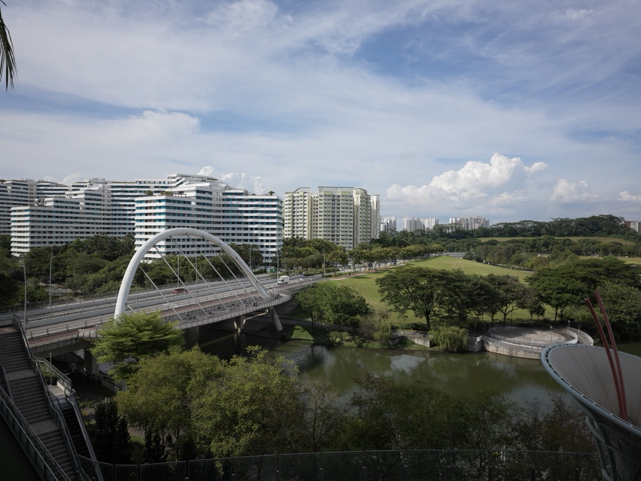
The Hydrology subject guide provides the foundation in catchments, streamflow and water accounting. Here the focus is experimental reasoning at catchment scale. All numerical records are invented. They do not evaluate an actual land-management scheme or the Punggol waterway shown in the contextual photograph.
eduKateSG · Hydrology
Choose the question closest to yours
Define the outcome, build the pre-intervention comparison, estimate a counterfactual and test how reference changes alter the causal claim.
Define the counterfactual · Chapters 1–2.
Calibrate and estimate · Chapters 3–5.
Convert and challenge the inference · Chapters 6–8.
Transfer to other water outcomes · Chapters 9–10.
Practise and check · Chapters 11–12.
Full chapter index · Subject foundation · Learning that transfers into life
Chapter contents
Define the counterfactual · Chapters 1–2
Calibrate and estimate · Chapters 3–5
Convert and challenge the inference · Chapters 6–8
Transfer to other water outcomes · Chapters 9–10
Practise and check · Chapters 11–12
CHAPTER 1 OF 12 · Define the counterfactual
1. Ask a question that names the outcome
Begin with a specific claim: did an intervention change annual runoff depth in catchment T during the first three complete post-intervention years? This question names the place, quantity and period. It is more answerable than “did the project improve the river?”, which combines several possible outcomes without defining any of them.
Annual runoff depth expresses outflow volume relative to catchment area. It helps compare differently sized catchments when that normalisation fits the question. It is not the same as peak discharge, a low-flow statistic, sediment load or water quality. An intervention may affect these outcomes differently.
Specify the intervention too. The timing, area affected and actual work completed matter. A plan for planting, drainage repair or forestry management is different from the intervention delivered on the ground. The study’s evidence should describe the actual change rather than attach all later differences to a project title.
Choose the comparison period before inspecting favourable results. Different periods can produce different estimates because weather and catchment responses vary. A transparent analysis explains why the window answers the question and reports important departures or missing periods rather than quietly dropping inconvenient years.
For a student, the first practical task is to rewrite a broad claim as a measurable question. Name one outcome and one period. Then list the other outcomes that the proposed study would leave unresolved. This boundary-setting makes the later calculation more useful because the reader knows what it is supposed to establish.
CHAPTER 2 OF 12 · Define the counterfactual
2. Understand why before-and-after is insufficient
Suppose catchment T averaged 250 mm annual runoff before an intervention and 140 mm afterwards. The observed change is −110 mm. That is a valid description of the supplied periods. It is not yet an estimate of the intervention’s effect because other conditions may also have changed.
Rainfall, atmospheric demand, storage carried from earlier years and other influences can alter streamflow. Some influences may affect neighbouring catchments together. Others may act differently because the catchments have different soils, geology or drainage arrangements. A simple temporal contrast has no direct way to separate these explanations.
The counterfactual question is: what would T’s runoff have been in the later years if the intervention had not occurred? We cannot observe that alternative history directly for the same catchment. A reference catchment and a pre-intervention relationship can provide evidence for estimating it under explicit assumptions.
This does not make the reference a perfect duplicate. The method can work with catchments that differ consistently. Its usefulness depends on whether their measured relationship is sufficiently stable and informative for the comparison. Two neighbouring catchments with similar names are not automatically a valid pair.
The Forest Service overview of paired-watershed studies places such experiments within long-term hydrological research. Our invented example uses that comparison logic without claiming that its simple equation is a validated model for any actual watershed.
CHAPTER 3 OF 12 · Calibrate and estimate
3. Establish the comparison before intervention
Call the reference catchment C and the intervention catchment T. Monitor them concurrently before the intervention, using compatible periods, quantities and measurement practices. The pre-intervention period is often called calibration: it establishes the relationship used to predict T from C in the example.
The reference should remain free of the intervention being evaluated. It also needs monitoring for other meaningful changes. An unrecorded abstraction, drainage alteration, disturbance or instrument replacement can undermine its role as a comparator even if the original project never touched it.
Site differences should be documented rather than hidden. Area, rainfall exposure, soils, groundwater connections, land cover and existing regulation can affect how the catchments respond. A strong relationship during a few similar years may not remain reliable across a much wider range of conditions.
Keep the measurement pathway visible. Streamflow may be derived from water levels through a rating relationship; changes in the channel or monitoring arrangement can change that conversion. A sudden difference in derived runoff may therefore come from measurement comparability rather than the land intervention.
The Forest Service calibration study examines stability in pre-treatment relationships. The general lesson for the learner is to inspect whether the comparison was stable enough to support the intended estimate. Calling a period “calibration” does not make every event within it free from other influences.
CHAPTER 4 OF 12 · Calibrate and estimate
4. Build an original calibration relationship
For the first teaching model, use four fictional complete pre-intervention years. Both columns contain runoff depth over the same annual periods. The values are deliberately exact so the relationship can be derived without statistical software.
| Pre-intervention year | Reference C, mm | Catchment T, mm |
|---|---|---|
| 1 | 100 | 130 |
| 2 | 200 | 210 |
| 3 | 300 | 290 |
| 4 | 400 | 370 |
When C increases by 100 mm, T increases by 80 mm. The slope is therefore 80/100 = 0.8. Substitute the first row into T = a + 0.8C: 130 = a + 80, so a = 50. Our invented pre-intervention relationship is T = 50 + 0.8C.
Check another row independently. For C = 300 mm, predicted T is 50 + 0.8 × 300 = 290 mm, matching the table. Check all four rows before using the equation. This catches an intercept or copying error while the model remains easy to inspect.
The intercept is part of this fitted teaching relationship, not a claim that a catchment can generate water from nothing when C is zero. The data cover C from 100 to 400 mm. Applying the line at zero or far outside that range adds an extrapolation not supported by these four rows.
Nor do four exact points prove that real catchments respond without noise. The model isolates the logic of predicting one series from another. Real calibration requires enough appropriate observations, attention to dependence and seasonality, and an uncertainty analysis suited to the actual record.
CHAPTER 5 OF 12 · Calibrate and estimate
5. Predict the unobserved comparison and calculate the departure
Now suppose the intervention has occurred in T, and three subsequent years yield the following fictional observations. Use the earlier equation to estimate T’s runoff under the assumption that its pre-intervention relationship with C would otherwise have continued.
| Post-intervention year | Reference C, mm | Expected T, mm | Observed T, mm | Observed minus expected, mm |
|---|---|---|---|---|
| 5 | 150 | 170 | 140 | −30 |
| 6 | 250 | 250 | 220 | −30 |
| 7 | 350 | 330 | 300 | −30 |
For year 5, expected T is 50 + 0.8 × 150 = 170 mm. Observed T is 140 mm, giving a departure of 140 − 170 = −30 mm. The other two years yield the same departure. Under this model, T produced 30 mm less annual runoff than its reference-based expectation in each post-intervention year.
The sign convention matters. We use observed minus expected, so a negative value means below the modelled counterfactual. A report using expected minus observed would give positive 30 mm for the same shortfall. State the convention instead of assuming that every positive number represents an increase in flow.
The post-intervention observed mean is 220 mm and the expected mean is 250 mm. Their difference is again −30 mm. This is the mean modelled departure over the three specified years. It is not automatically the permanent annual effect, nor does it identify the physical pathway responsible.
CHAPTER 6 OF 12 · Convert and challenge the inference
6. Compare the result with a misleading temporal contrast
Our four calibration years have a mean C of 250 mm and mean T of 250 mm. The three post-intervention years also have mean C of 250 mm, but mean observed T of 220 mm. In this particular balanced example, a before-and-after mean happens to agree with the reference-adjusted departure.
Now change the post-intervention sample to a single dry year with C = 100 mm and observed T = 100 mm. The pre-intervention relationship predicts T = 130 mm, so the modelled departure remains −30 mm. Yet a raw comparison with the earlier T mean gives 100 − 250 = −150 mm.
The additional −120 mm in the raw contrast reflects the different reference conditions under the teaching model. Without the concurrent comparison, it would be easy to attach the entire −150 mm change to the intervention. The paired approach asks a more specific question about departure from the expected response in that dry year.
Now choose a wet post-intervention year with C = 400 mm and observed T = 340 mm. The raw comparison gives 340 − 250 = +90 mm, suggesting increased runoff. The expected T is 370 mm, so the modelled departure is still −30 mm. A temporal increase and a negative intervention-related departure can coexist.
This pair of changed-context examples is worth explaining aloud. The intervention estimate is not simply the direction in which the observed series moved. It depends on the comparison with a defensible expectation for the same later conditions. That is the central counterfactual idea.
CHAPTER 7 OF 12 · Convert and challenge the inference
7. Translate depth into volume without changing the claim
Suppose T has a contributing area of 2 km² for this exercise. A modelled annual departure of −30 mm corresponds to −0.030 m × 2,000,000 m² = −60,000 m³. The negative sign retains our observed-minus-expected convention.
This conversion changes units, not evidential strength. A large-looking volume does not make the causal attribution more certain. It also does not establish that 60,000 m³ was available for a particular use, stored permanently underground or removed from flood peaks. Those are separate claims requiring additional evidence.
Check the physical quantity carefully. Millimetres of runoff depth already represent volume divided by catchment area. Multiplying by area restores volume. Multiplying by time again would be wrong unless the original quantity were a rate requiring integration. Unit control prevents a meaningful comparison from turning into a dimensional error.
For three annual departures of −30 mm each, the cumulative modelled departure is −90 mm, corresponding to −180,000 m³ over the three-year window at the same area. This sum assumes the three annual quantities are compatible and does not by itself describe the final storage state at the end of year 7.
The independent check is to calculate each year’s volume separately and add them. Then compare with the cumulative-depth calculation. Agreement verifies the arithmetic and units. It does not independently verify the counterfactual model, because both routes use the same estimated departures.
CHAPTER 8 OF 12 · Convert and challenge the inference
8. Inspect uncertainty rather than celebrating exact residuals
The repeated −30 mm values were constructed to make the reasoning visible. Real observations would scatter around the calibration line, and the estimated slope and intercept would be uncertain. Measurement error and natural variability also affect the departure. A point estimate should therefore remain connected with its uncertainty.
Imagine that an appropriate analysis produced a prediction interval for one year’s untreated T response from 150 to 210 mm. An observed value of 140 mm would be below that interval. If the interval were instead 110 to 230 mm, the same observation would be less distinctive. These are illustrative intervals, not intervals fitted from our four exact calibration points.
Distinguish an interval for the expected mean relationship from a prediction interval for an individual future year. The latter includes additional year-to-year variation. Using the narrower mean interval to judge a single observed year can exaggerate confidence in a departure.
Consecutive daily or monthly values may be dependent. Treating every reading as an independent replicate can overstate effective sample size. Likewise, three post-intervention years in one treated catchment are not three independently assigned catchment interventions. Temporal replication and replication of treatment units are different forms of evidence.
The practical reporting question is whether the estimated departure is large and persistent relative to the relevant uncertainty, and whether alternative explanations have been investigated. A sophisticated significance label cannot substitute for a stable comparator and a clear account of what changed at the sites.
CHAPTER 9 OF 12 · Transfer to other water outcomes
9. Test the reference and the causal interpretation
Suppose C undergoes an unrecorded diversion after year 4 and reports 50 mm less runoff than it otherwise would. Using that reduced C in T = 50 + 0.8C lowers the predicted T by 40 mm. The apparent departure in T therefore shifts upward by 40 mm even if nothing has changed in T.
This numerical sensitivity shows why the control cannot be treated as background scenery. The reference produces part of the expected value. A meaningful change in C can alter the estimated effect attributed to T. Monitoring both catchments’ histories is essential to the comparison.
The Forest Service study of paired-watershed consistency examines how relationships can differ across periods. The lesson is not that paired comparisons always fail. It is that their identifying assumption—the continued usefulness of the calibrated relationship—needs examination rather than being hidden beneath the regression equation.
Causal confidence also depends on the study design. A deliberately timed intervention, careful controls and several independent pairs can support stronger inference than a retrospective comparison selected after a striking result. Random assignment, where feasible, addresses additional sources of systematic difference, but it does not remove every measurement or interpretation problem.
Write an explicit conditional conclusion: “T was 30 mm below the reference-based expectation; interpreting this as an intervention effect assumes the calibrated relationship would otherwise have persisted and no competing changes explain the departure.” The qualification tells the reader which evidence would strengthen or weaken the inference.
CHAPTER 10 OF 12 · Transfer to other water outcomes
10. Transfer from annual yield to peaks and water quality
Now ask whether a lower annual runoff depth proves that flood peaks fell. It does not. Annual yield sums water over a year. Peak discharge describes a maximum rate over a much shorter interval. Many different hydrographs can carry the same volume, and lower total volume can coexist with a higher short peak.
Construct an extreme invented comparison: one event conveys 1,000 m³ evenly over an hour, while another conveys 800 m³ concentrated into ten minutes at a constant rate during that interval. The first rate is approximately 0.278 m³/s; the second is approximately 1.333 m³/s. The smaller volume has the larger rate in this simple example.
A paired study of peaks would need appropriate event definitions, observation frequency, rainfall comparison and a model suited to peaks. The annual calibration cannot be reused solely because both outcomes involve water. The measured quantity and the time scale must match the claim.
Water quality introduces another distinction. A reduced concentration does not necessarily mean a reduced load if flow increases, and a reduced annual flow does not establish improved ecological conditions. Sampling timing, transported mass, habitat and the chosen outcome all matter.
The hydrograph-separation guide asks how a measured total is partitioned into inferred components. The flow-duration guide asks what sorting retains and hides. Read them beside this study design to keep components, frequency, chronology and causal attribution distinct.
CHAPTER 11 OF 12 · Practise and check
11. Practise a new calibration and plan better evidence
Try a second invented relationship: before intervention, T = 20 + 1.2C over the range C = 100–300 mm. In a later year C is 200 mm and T is observed at 245 mm. The expected T is 20 + 1.2 × 200 = 260 mm. The modelled departure is −15 mm.
Now change C to 500 mm while retaining the equation. A numerical prediction of 620 mm is easy to calculate, but 500 mm lies outside the calibration range. The arithmetic does not establish that the relationship remains valid there. The interpretation should flag extrapolation and seek evidence for behaviour under those conditions.
If the post-intervention period contains unusually wet extremes, one useful improvement is a longer calibration record spanning a wider relevant range. Other improvements may include independent comparison catchments, stable monitoring, rainfall observations and a documented intervention history. Choose the addition according to the weakness it would address.
A complete evidence record includes the outcome definition, site boundaries, monitoring methods, calibration window, model, diagnostics, intervention timing, post-intervention observations, uncertainty and competing changes. It should distinguish an observed difference from a modelled departure and from the further causal interpretation.
For a delayed transfer exercise, replace “catchment” with a fictional classroom programme and “reference runoff” with a suitable comparison measure. Ask which parts of the logic remain and which assumptions need to be rebuilt. The goal is not to copy a hydrological equation into education. It is to recognise why a before-and-after improvement needs a credible comparison before it becomes an intervention claim.
A final check concerns how an average effect is presented. Our three invented years each have a −30 mm departure, so their mean is transparent. A different study could have departures of −90, +20 and −20 mm, which also average −30 mm. The common mean would conceal a much less uniform annual pattern. Report the individual periods alongside a summary when that variation matters to the reader’s decision.
Next ask whether the same intervention effect is expected to persist. Vegetation, soil conditions and management can evolve after an intervention, while weather can move outside the range previously observed. A first-three-years estimate is not automatically a lifetime effect. Continuing measurement can reveal whether the departure persists, changes or becomes difficult to distinguish from other variation.
For a compact communication exercise, compare two headlines: “The project saved 60,000 cubic metres every year” and “Runoff was 60,000 cubic metres below the modelled annual expectation in the stated three-year study window.” The second retains the quantity, comparison and period. Neither headline alone establishes where the difference went or whether it improved water availability for users.
That last distinction matters. Lower runoff may correspond to changes in evapotranspiration, storage or other pathways, depending on the actual system. A catchment outflow departure is not a direct measurement of each pathway. To explain the mechanism, connect additional observations with a suitable water budget rather than assigning the entire residual to whichever process best fits the project narrative.
Must paired catchments be identical?
No. The approach uses a predictable relationship, not literal identity. Differences must be understood well enough that the calibration remains informative for the later comparison. Physical similarity alone does not prove that condition.
Is a reference catchment the same as untreated nature?
It is a comparison site whose relevant conditions should remain suitable for the study. Existing management, regulation and other activities must be documented. The word reference does not mean the site has never been altered.
Does a negative residual prove the intervention reduced flow?
It shows flow below the modelled expectation under the stated sign convention. A causal interpretation additionally depends on design, measurement comparability, uncertainty and the absence of competing explanations that account for the departure.
Why not use a simple before-and-after mean?
A temporal contrast combines the intervention with other changes across periods. Our dry-year and wet-year examples show how the raw change can exaggerate or even reverse the impression created by the reference-adjusted comparison.
Can a good annual model establish lower flood risk?
No. Annual volume and short-duration peaks are different outcomes. Flood consequences also depend on exposure and vulnerability. A separate analysis should use observations and methods matched to the risk question.
Is more frequent measurement always more replication?
It adds temporal detail, which can be valuable. It does not create additional independently treated catchments, and dependent observations should not be counted as if every reading were independent evidence of an effect.
What is the clearest final sentence?
State the observed departure, the outcome and period, the counterfactual model and the main attribution assumption. That lets a reader understand both what changed in the evidence and what remains conditional in its explanation.
Continue through the connected guides
Compare a connected investigation
Inspect measurement consistency before treating a departure from a calibrated relationship as evidence of an intervention. Continue with The Gold Standard of Hydrology | Double-Mass Curves and Rain-Gauge Consistency.
Measurements, summaries and inferred components
The Hydrology root guide connects rainfall, storage, catchments and water accounting. The hydrograph-separation article distinguishes a measured total from a modelled partition. The flow-duration article distinguishes frequency from chronology. Read them together when deciding which features of a record a particular method preserves.
Evidence and practical water decisions
The environmental laboratory testing guide follows representative samples and clear reporting limits. The water-quality monitoring guide connects observations with the question they can answer. The water-resources engineering guide carries water estimates toward planning and community needs. None of these applications can be established by a tidy graph alone.
Mechanisms, restoration and transfer
The groundwater investigation guide examines subsurface pathways. The river-restoration guide connects interventions with functioning systems and evidence of recovery. Continue through the education parent for learning that transfers, or the How X Works hub to compare how evidence is used in other subjects.
Sources and scope
The Forest Service records for paired-watershed calibration, consistency of hydrological relationships and past and future roles of paired watersheds support the study-design context and the importance of stable comparison relationships.
All calibration values, interventions, prediction intervals and sensitivity scenarios are original teaching examples. They do not constitute a fitted study, a real treatment-effect estimate or a design recommendation. The photograph shows Punggol Waterway Park as a contextual urban water setting, not a monitored experimental pair.
The numerical datasets and classroom scenarios in the worked examples are invented for learning. Sources were checked on 21 October 2026. “Gold standard” describes the educational benchmark explained here; it is not an accreditation.
Hydrology root guide · The Gold Standard of Education · Explore How X Works