
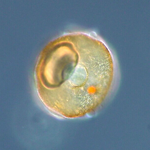
Testate amoebae analysis uses preserved microscopic shells in peat and other wetland deposits to study past hydrological conditions. A change in their assemblages can support an interpretation that a bog became relatively wetter or drier, but it does not automatically supply an exact water-table depth or prove a specific drought. Responsible teaching combines morphological identification, modern ecological calibration, chronology and model uncertainty.
This complete reference explains shells, peatland microtopography, Arcella identification, water-table depth, species- and trait-based transfer functions, validation and an invented Larch Fen calculation. The featured photograph is a real modern Arcella testate amoeba from a pond in Japan, not a fossil from Larch Fen. The objective is to help learners calculate and interpret evidence without confusing an appealing numerical reconstruction with an independent water-level measurement.
The Central Sumatra calibration study and independent modern-water-table validation illustrate the promise of the method and the importance of carefully limiting claims.


1. What the shells can tell us about a bog
Testate amoebae are single-celled organisms that occupy protective shells called tests. Their communities live in wetlands, mosses, soils and other environments, and many peatland taxa respond to water availability and chemistry. Fossil tests preserved in peat can therefore contribute evidence about past hydrological conditions. The strongest claim is often a shift towards wetter or drier bog surfaces under a stated method, not an exact reconstruction of rainfall, a specific flood or the water table on one historical morning.
Begin with a microscope photograph of a genuine modern Arcella shell, then introduce an invented peat core. Ask learners to distinguish the directly observed shell from the ecological inference that follows. A test is not a rainfall gauge. It records an organism’s response to a range of conditions, later filtered through peat accumulation, burial and laboratory recovery. The learning objective is to connect those processes before reading a reconstructed water-table curve.
2. Explain what the term testate amoebae includes
The familiar term describes several groups of shelled amoeboid protists rather than one simple, uniformly related family. Tests may be secreted from organic or mineral materials, or assembled from particles collected from the environment. Shape, aperture, size and construction can aid identification. Students should not confuse these shells with pollen grains, tiny animal eggs or foraminiferal tests merely because all can appear in a microscope slide. The taxonomic context determines what environmental interpretation is appropriate.
Have learners draw a round test, an elongated test and one built of agglutinated particles. Label the aperture and possible surface structures. They must identify what can and cannot be resolved without further magnification or comparative references. A high-quality response may assign one fossil only to a broad morphotype when its diagnostic features are damaged. Confidence should respond to the surviving morphology, not to the ambition of the climate story.
3. Separate the living cell from the preserved test
The living amoeboid cell performs metabolism and may extend pseudopodia through the aperture. After death or environmental stress, the durable test may remain in sediment while soft parts do not. The test is consequently a useful fossil structure, but its abundance depends on production, preservation and transport. One shell may represent one individual structure, yet a recovered test assemblage is not necessarily a random census of every living organism that once occupied a moss surface.
Use an illustrated life-history diagram to distinguish organism, test, fossil test and sorted laboratory observation. Then ask learners how partial breakage, selective recovery or sediment mixing could change the apparent community. Their written description should name the object actually counted. This develops the same methodological caution used in studies of diatoms, charcoal and other fossil microremains.
4. Define peatland hydrology carefully
Peatlands can be rain-fed, groundwater-influenced or connected to other surface-water systems. In raised rain-fed bogs, local moisture conditions may be closely tied to climatic water balance, but plants, microtopography and evaporation also matter. Water-table depth is commonly expressed as the distance below a reference surface, though the sign convention must be made explicit. A deeper water table often indicates relatively drier surface conditions, but a number is meaningful only when its measurement method and reference are known.
Set up a conceptual transect with a raised hummock, a lawn and a wet hollow. Measure depth relative to each local surface rather than treating the whole bog as a bathtub with one universal level. Students should explain why a nominal water-table depth of twenty centimetres under one microform may not represent the same biological moisture exposure as twenty centimetres elsewhere. This prepares them for calibrated ecological comparisons.
5. Recognise hummocks, lawns and hollows
The surface of many bogs is structured by small-scale elevations, moss growth and wet depressions. Testate amoeba communities can differ strongly among these microhabitats even within one peatland. A sampling programme that compares modern hummocks with fossil material deposited primarily in hollows may mistake a microtopographic difference for a climatic change. Published work on bog microtopography shows that responses to weather vary between microforms and cannot be assumed identical.
Ask students to design a field map with multiple sampling points across hummocks, lawns and hollows. Each point needs an elevation reference, vegetation notes and water-table measurement. A single visually representative surface sample is not always enough. The best learners describe how their spatial design helps separate local habitat effects from a broader hydrological signal.
6. Identify Arcella and its relatives with reference care
Arcella often has a rounded test with a characteristic aperture, while other common testate amoebae may show distinctly different shapes and shell materials. Nonetheless, diagnostic detail varies among species and preservation states. The featured photograph here shows a modern Arcella specimen photographed in Japan. It is not a fossil from the fictional Larch Fen core, and the image alone cannot determine the ecology of every Arcella morphotype around the world.
Set students an identification exercise using images from verified modern reference collections. Require a scale, viewpoint, aperture location and note about test construction. If a fossil cannot be identified beyond an Arcella-like group, that uncertainty should appear in the dataset. The skill being taught is evidence-based morphology, not the memorisation of a photograph that becomes an unreliable identification shortcut.
7. Include agglutinated and secreted test materials
Some testate amoebae build shells by binding external mineral or biological particles, whereas others form tests largely from material produced by the organism. Substrate availability can influence the resulting test appearance. Fragile organic tests and mineral-rich tests may survive differently during burial or laboratory processing. Therefore, an apparent shift in test types could reflect environmental change, but also differential preservation or sediment supply.
Give students two fictional slides with different sediment mineral fractions and ask why a test built of coarse grains might stand out in one but be partly obscured in another. They must separate organism-level morphology from changes caused by preparation. It is worth teaching this before a data model treats every apparent taxonomic change as a climate event.
8. Use a standardised field and subsampling protocol
Modern calibration and fossil reconstruction require carefully documented sampling. Field records should include site, coordinates, microform, vegetation, recent moisture conditions, depth, sample volume or mass and laboratory handling. A peat core must preserve the order of layers and avoid confusing neighbouring depth intervals. Where contamination or disturbance occurs, the record should say so. The procedural details allow different researchers to understand what the counts represent.
Ask a group to create a specimen card for each sample in a hypothetical Larch Fen transect. Deliberately remove one depth label and one microtopographic description from a second set. Students should identify which later comparisons are weakened and why the missing fields cannot simply be reconstructed from a convenient graph. Reproducibility begins before the microscope.
9. Distinguish modern training sets from fossil cores
A modern training set links identified living or recently deposited assemblages to environmental measurements, often water-table depth, pH, moss moisture and vegetation conditions. A fossil core provides assemblages from older sedimentary layers where the environmental values must be inferred. A transfer function is a statistical relationship derived from the modern observations and applied to the older assemblage. It is not a direct physical measurement of past water depth.
Students should draw two parallel diagrams. The modern side contains both taxa and observed hydrological measurements; the fossil side has taxa and age-depth information but unknown hydrology. An arrow marked ‘model with assumptions’ connects them. This diagram is more important than memorising a software command because it makes clear what evidence the reconstruction gains—and what it continues to assume.
10. Explain why the geographical calibration matters
Taxa found in a peatland in western Europe may not have identical observed relationships with hydrology in tropical Indonesia, Siberian permafrost or an Australian high-altitude mire. Differences in communities, habitat, vegetation and water chemistry make direct model transfer risky. The 2020 Sumatra study developed region-specific relationships using both species composition and functional traits, illustrating that modern data from the appropriate environment can be more defensible than borrowing a distant model unchanged.
Ask learners to examine the location and ecological scope of any published transfer function before applying it. A model can perform well statistically in its own region yet lack good analogues for a new peatland. The lesson should require students to ask which species are present in both sets, whether their environmental ranges overlap and whether the modern sites sample the full gradients represented by the fossils.
11. Learn how water-table depth and pH interact
Testate amoeba assemblages can respond to hydrology, pH and other environmental factors at the same time. Modern observational correlations may not show a unique causal mechanism. In one calibration set, water-table depth might dominate the measured gradient; in another, acidity and vegetation could contribute substantially. It is a mistake to interpret every change in a named taxon as a linear response to water depth while ignoring the chemistry of its habitat.
Design a matrix in which two sites share an observed water-table depth but differ in pH and moss composition. Ask whether identical testate assemblages must follow. Students should propose measurements that can help distinguish hydrology from other environmental effects. A strong report explicitly describes which predictors were measured and which potential confounders were not.
12. Understand species-based and trait-based approaches
Species-based reconstruction models use identified taxa and their observed distributions, while trait-based models can represent features such as shell width, shape and aperture geometry. Both have strengths and limitations. Traits may permit ecological comparisons when taxonomy is uncertain, but a trait is not necessarily unique to one response. The Sumatra research evaluated both approaches and discussed how regional species composition influences model development.
Students can build a toy trait table containing test width, test compression and aperture type, then compare it with a taxon frequency table. They should ask which information survives a partially damaged fossil and which uncertainties are introduced by recording traits. The correct conclusion may depend on the research question, sample quality and the calibration design rather than declaring one approach universally superior.
13. Introduce weighted averaging without magic
A simple weighted-average reconstruction associates each taxon with an optimum along a measured environmental gradient, then weights those optima by their observed abundance in a fossil sample. This makes an intuitive classroom model, but genuine transfer functions need calibration choices, transformations, taxonomic consistency, error estimates and independent evaluation. No student should mistake a spreadsheet average of made-up optima for a scientifically validated estimate of past water-table depth.
In the fictional Larch Fen exercise, three morphotypes are assigned toy modern optima of ten, twenty and forty centimetres below the moss surface. Their values are invented for arithmetic practice. Learners calculate a weighted score from frequencies, then identify why the resulting number cannot become an actual historical water-level measurement without a proper modern calibration and validation.
14. Calculate the fictional Larch Fen sample A
Imagine fossil sample A contains twenty counts of morphotype One, sixty of Two and twenty of Three, with the invented optimum depths of ten, twenty and forty centimetres respectively. A naive weighted-average score is (20 × 10 + 60 × 20 + 20 × 40) / 100 = twenty-two centimetres. The expression is dimensionally sensible for a simplified classroom demonstration but lacks a real transfer-function correction, observational uncertainty and regional calibration.
Ask students to show every term in the numerator and explain why the denominator is the total confidently classified test count. If some tests were unknown, their treatment should be documented rather than silently redistributed. Then ask what would change if the known taxa were poor modern analogues for this peat core. A correct calculation and a defensible environmental reconstruction are related but distinct accomplishments.
Fictional Larch Fen weighted-average exercise
| Morphotype | Toy optimum below surface | Sample A count | Sample B count |
|---|---|---|---|
| One | 10 cm | 20 | 60 |
| Two | 20 cm | 60 | 30 |
| Three | 40 cm | 20 | 10 |
| Toy weighted score | Not a calibrated measurement | 22 cm | 16 cm |
15. Calculate the fictional Larch Fen sample B
Fictional sample B contains sixty counts of morphotype One, thirty of Two and ten of Three. The same toy formula gives (60 × 10 + 30 × 20 + 10 × 40) / 100 = sixteen centimetres. Under the invented optima and the stated downward-positive depth convention, this is six centimetres shallower than sample A. That directional difference might suggest wetter conditions in a validated context, but the numbers are not predictions for any real bog.
Have learners calculate percentages and confirm that the weights sum to one hundred for each sample. They should then test how much the difference changes if several marginal tests are reclassified. The exercise is designed to introduce sensitivity and numerical literacy before more sophisticated modelling, not to create a falsely precise palaeoclimate graph.
16. Respect model errors and root mean squared prediction error
Model performance is often described with statistics such as root mean squared error of prediction, abbreviated RMSEP, and measures of explained variation. These summarise predictive performance under a particular validation scheme; they do not guarantee the error for every fossil sample. A published model may have errors of several centimetres while individual reconstructions are more uncertain because of poor analogues, unusual ecology or measurement mismatch.
Give students a hypothetical model RMSEP of six centimetres and a toy difference of six centimetres between reconstructed samples. Ask whether they can confidently announce a six-centimetre historical change. They should consider covariance, chronology, uncertainty structure and whether the model has been validated in a comparable environment. An impressive precision statistic cannot replace a discussion of the actual inference being made.
17. Understand cross-validation and spatial autocorrelation
Leave-one-out cross-validation can test a model by predicting each modern observation while excluding it from fitting. However, nearby samples may share environmental and biological characteristics, making simple random or leave-one-out tests overly optimistic when spatial dependence is strong. Leave-one-site-out or geographically structured testing may provide a more demanding assessment of portability. Model design must match the inference a researcher intends to make.
Have learners divide a hypothetical calibration set into two peatlands. A model tested only on nearby samples may look accurate because those samples resemble its training data. Ask whether it remains accurate when the entire second site is withheld. This is an advanced but practical lesson: the quality of validation depends on the independence of the test, not just on the number reported in a methods table.
18. Check for non-analogue fossil communities
A fossil assemblage may contain taxa or trait combinations poorly represented in the modern training set. In that case, even a polished transfer function may be extrapolating beyond the environments used to build it. Dissimilarity metrics and analogue tests can flag this problem. A poor analogue should not be hidden behind a plotted number; it is a reason to widen the calibration, revise taxonomic harmonisation or narrow the claim.
Give the class a fossil assemblage dominated by a morphotype nearly absent from the modern reference. Learners should flag the unsupported part of the reconstruction and recommend follow-up modern sampling or a more cautious qualitative assessment. The correct skill is recognising a model’s domain of applicability. Mathematics cannot manufacture modern ecological evidence that was never collected.
19. Distinguish directional change from an exact baseline
Independent monitoring work has found that testate amoeba transfer functions can capture directional hydrological changes yet be poor representations of measured mean or median water-table magnitudes at particular sites. This is a crucial teaching distinction. A reconstruction may be useful for identifying a wetter interval relative to an earlier one without providing the absolute centimetre value a contemporary land manager would need for restoration decisions.
Ask students to rewrite an overconfident sentence stating that a historical bog’s water table was exactly twenty-two centimetres below ground. A better report explains that, under the stated model and relative reference, assemblage shifts are consistent with deeper or shallower local water-table conditions, with specified uncertainty. The learning goal is useful environmental interpretation without a fabricated level of precision.
20. Treat depth as time only after building chronology
A peat core records material by depth, while its time interpretation depends on appropriate dating and age-depth modelling. Different accumulation rates, hiatuses, decomposition and disturbance can affect the relationship. A change between adjacent centimetres may represent an unequal number of years. A fine-grained graph cannot legitimately assign an exact historical year unless chronology supports that resolution.
Offer two core segments with the same thickness but different modelled durations. Students must decide whether the differences could be related to one documentary drought. A scientifically cautious report states the date range and uncertainty. It should not confuse a sample’s physical depth with the date of the ecological conditions inferred from its shell assemblage.
21. Understand peat decomposition and selective test survival
Peat decomposition changes organic matter, physical structure and the preservation of small organisms. Some tests may remain identifiable while others are preferentially damaged or removed, affecting observed assemblages. Chemical treatments, storage and mechanical processing can also change what the analyst sees. These factors need to be considered alongside real ecological change, especially when comparing cores collected or processed by different teams.
In a fictional sample pair, one interval has heavily damaged thin-walled tests and many indeterminate fragments. Students calculate taxon proportions only after documenting the missing and uncertain categories. They then ask whether the shift could be explained by different survival rather than a drier climate. Quantification without a preservation audit can convert a laboratory artefact into a plausible climate narrative.
22. Compare testate amoebae with plant macrofossils
Peatland plant macrofossils and testate amoebae provide different hydrological clues because plants and protists respond through distinct physiological and ecological pathways. Comparative studies in Finland and Estonia have found broadly similar long-term trends but also episodes of disagreement. These disagreements can reveal differences in sensitivity, habitat structure, chronology or calibration. Independent proxies improve reasoning when their assumptions are examined rather than simply averaged.
Present a hypothetical layer where plant remains suggest relatively dry conditions while testate amoebae suggest wetter conditions. Students must propose tests for preservation, local vegetation, taxonomic identification, sampling resolution and dating. The correct result may remain unresolved. The lesson is not to choose the proxy that creates the most convenient story but to use divergence as information about the system.
23. Avoid treating peatlands as pure climate gauges
A peatland’s hydrology may reflect precipitation and evaporation, but drainage, local vegetation change, peat growth, geomorphology and human land use can also affect water-table conditions. A reconstructed shift in local moisture cannot automatically be assigned to regional rainfall decline. Archaeological interpretation requires a causal argument that integrates land-use evidence and regional environmental context.
Ask learners to create competing explanations for a fictional drying signal: reduced precipitation, local drainage, increased evapotranspiration and changes in bog surface microtopography. They must identify which independent observations could discriminate them. A proxy is strongest when it helps narrow the set of possible histories, not when it becomes a single-answer machine.
24. Apply the method carefully in tropical peatlands
Scientific work in Central Sumatra demonstrates that testate amoeba morphotypes and functional traits can be calibrated against hydrology in tropical peatlands, with water-table depth and pH among the environmental variables considered. But the findings also underscore the need for region-specific models because species composition and environmental relationships differ across latitudes. Importing a European optimum table to an Indonesian peat swamp would be a hypothesis requiring testing, not a valid shortcut.
Have students plan a Southeast Asian calibration survey spanning a real water-table gradient and distinct vegetation zones. They need replicated locations, field water-level measurements, trait records and appropriate validation. Their proposal should acknowledge that water-table measurements made on one visit may not capture full seasonal hydrological behaviour. The task combines field design with statistical judgement.
25. Consider permafrost peatlands as a contrasting case
Cold-region peatlands introduce additional complexities involving freeze-thaw dynamics, vegetation microhabitats and changing water regimes. A 2023 study developed a regional testate amoeba hydrological transfer function for permafrost peatlands in northwestern Siberia and found that vegetation type influenced relationships with water-table depth. This makes an instructive contrast with rain-fed European bogs and tropical peat settings.
Ask students what the phrase ‘calibration is transferable’ would have to mean across these environments. They should compare organism communities, environmental gradients, seasonality, site history and independent field observations. A model is a scientific instrument built for particular conditions; responsible teaching asks learners to check those conditions before using its output as history.
26. Interpret findings alongside archaeology without inventing occupations
Peat and wetland records may be near prehistoric settlements, trackways, drainage structures or historical land-use zones. Their hydrological histories can contribute context for how people used landscapes. Nevertheless, an amoeba-derived wet phase does not prove a settlement was abandoned because of flooding, and a drier phase does not prove deliberate drainage. Such human-history claims need stratigraphic, chronological, artefactual or documentary evidence beyond the ecological proxy.
Give students a fictional timber trackway and a nearby peat core that may show a wetter interval. They must identify whether the dates overlap within uncertainty, whether the core reflects conditions at the trackway and what archaeological evidence exists for construction or abandonment. The lesson develops interdisciplinary reasoning without treating one graph as a human biography.
27. Teach reproducible microscopy and classification
A reliable lab report stores raw counts by morphotype, microscope settings, counted sediment or slide area, identification references, damaged tests, and photographs showing diagnostic features. Training and blind repeat counts can expose disagreements. Some morphotypes may be consistently recognisable, while others require a broader category. The data archive should keep original classification decisions and documented revisions.
Conduct a blind two-reader identification exercise with reference images. Students compare exact agreements and explain common errors rather than forcing a perfect score. The next step is to revise the identification guide and recount a subset. This improves the reproducibility of any later transfer-function reconstruction and helps learners see that model quality begins in taxonomic observation.
28. Show uncertainty in figures and conclusions
A published figure should indicate the actual sample positions, age ranges where applicable, analytical uncertainty and whether numerical values come from validated calibration or only descriptive indices. If a data point has a poor modern analogue, marking it can be more informative than hiding it. Smooth interpolation between sparse samples may look beautiful but can imply changes that were never directly observed.
Ask learners to redesign an exaggerated climate chart. The original has exact dates and two decimal places on water depth; the revised version shows samples, model limitations and the distinction between relative hydrological trend and absolute estimate. A strong figure communicates what the data permit without sacrificing readability.
29. Build a scientific assessment that rewards caution
Assess learners on identification, ecological reasoning, mathematical accuracy, model validation, preservation control and clear evidence-limited interpretation. The highest-quality answers state both what the shells suggest and what other causes could produce a similar assemblage shift. A sophisticated student may say that the local record supports changing moisture conditions but cannot isolate the contribution of regional climate from drainage or vegetation dynamics.
Use a final audit in which students identify one unsupported causal phrase and rewrite it into a testable statement. They should propose specific follow-up evidence rather than merely adding vague disclaimers. The gold standard is a useful result that another researcher can independently understand, reproduce and challenge.
Twenty advanced classroom and research audits
Every case below is hypothetical. The purpose is to train scientific judgement and ensure that calculations are not mistaken for real palaeohydrological measurements.
1. A broken Arcella shell
A learner examines a fragmentary rounded test with a missing aperture. The shape resembles Arcella, but diagnostic features are incomplete. Ask whether the specimen can support species-level identification or should remain a broader morphotype. Students must record scale, preservation and a comparable modern reference before allowing the specimen to enter a species-specific calibration table.
2. The hummock-hollow mismatch
A modern calibration was built from hummocks, but a fossil core seems to contain assemblages more typical of wet hollows. Students evaluate whether the model’s environmental and microtopographic range covers the fossil community. They propose expanding the training set or reducing the certainty of the reconstruction rather than pretending that the same taxon has an identical moisture optimum in every microhabitat.
3. The invented exact water table
A textbook example reports a reconstructed twenty-two centimetre depth from uncalibrated optima. Students verify the weighted average and then explain why the output is not a measured historic level. They must name the missing elements: modern training data, validation, analogue testing, chronostratigraphy and uncertainty. The exercise rewards correctly limiting a calculated answer.
4. Taxonomic confusion
A pollen grain, a diatom and an amoeba test are deliberately mixed in a slide set. Learners must identify what supports each classification and preserve indeterminate objects. They should not label every circular outline a testate amoeba. The goal is to build morphology-based reasoning before an environmental model converts errors into a hydrological narrative.
5. The peat core without dates
A testate assemblage shift occurs thirty centimetres below the top of a peat core. A student assigns it a famous drought year with no age model. The group proposes dating control and stratigraphic evaluation and writes a depth-specific interpretation first. They should learn that ecological evidence and chronology are separate measurements that must be connected explicitly.
6. The spatial autocorrelation trap
One hundred calibration samples come from ten closely packed sites. A leave-one-out score looks very strong. Students test a leave-one-site-out approach and discuss why the result may be less impressive but more relevant to transfer beyond the sampled site. This exercise helps them understand what validation independence means, not just how to quote a model statistic.
7. A shallow water table but dry moss
Two places share similar recorded water-table depth during a field visit, yet local moss moisture differs because of microtopography and vegetation. Students investigate why one water-table measurement may not describe biological exposure. They propose repeated monitoring and vegetation notes and explain how such conditions could complicate fossil taxon interpretation.
8. The non-analogue fossil
An old peat sample contains a common fossil morphotype barely represented in the modern reference collection. Students mark the model prediction as questionable and design further modern sampling. A confident numeric answer without discussing the missing analogue is a lower-quality scientific result than a calibrated qualitative statement.
9. The two-proxy disagreement
Plant macrofossils suggest a relatively dry phase while testate amoebae suggest wet conditions. Teams list differences in ecological response, source area, preservation, taxonomic uncertainty and model calibration. Each proposes one independent test. Students should retain disagreement in the published record rather than deleting it to create a tidy climate story.
10. Damaged-test preservation bias
A sample has unusually few fragile organic tests but many robust mineral-rich tests. Students are asked whether the community changed or fossil survival changed. They inspect preservation notes and suggest controls before drawing an environmental conclusion. This exercise tests taphonomic reasoning, not the speed of a taxon percentage calculation.
11. The misplaced moisture sign
A student reports that water-table depth increased from ten to thirty centimetres below the surface and therefore the bog became wetter. The class checks the downward-positive convention and explains why deeper generally indicates a drier surface in the toy setting. Then they ask whether the actual ecology and calibration support the same directional interpretation.
12. An exaggerated climate claim
A reconstructed moisture decline is immediately labelled regional drought. Students list local drainage, vegetation and surface evolution as alternatives, then describe which independent climate or archaeological data would help. The exercise separates hydrological reconstruction from attribution and teaches why one proxy need not have one cause.
13. The inconsistent volume counts
One fossil sample is counted over a large processed volume while the comparison sample uses a small one. Students first verify raw taxon proportions and then discuss sampling effort, rare taxa and detection. They should identify which measures can reasonably be compared, especially when small totals exaggerate apparent ecological differences.
14. An Australian model used in Indonesia
A classmate downloads a high-performing model from a different hemisphere and applies it without checking taxa or environmental gradients. The peer-review group challenges analogue quality, trait comparability and regional hydrology. Their correction is to seek an appropriate calibration, not to assume the model is worthless everywhere.
15. A fragile cultural archive
A proposed classroom practical would consume the only undisturbed sample from a protected wetland archaeological feature. Learners weigh scientific benefit, permission and alternatives such as archived images or already prepared slides. A scientifically justified decision may be to preserve the original material. Research ethics are part of good evidence production.
16. The peer-review handover
A group receives only a smooth reconstructed curve, with no taxa, core depths, microscope logs or dating uncertainty. They must list the information needed to reproduce it. The class then writes a short required data and metadata checklist. The exercise makes the quality standard measurable: a finding that cannot be reconstructed from its own records has an avoidable weakness.
17. The functional-trait dispute
Two students disagree on whether to use a trait-based or species-based model after examining partially damaged tests. They design a comparison using appropriate reference data and validation, explaining which method tolerates their observed uncertainty. The correct answer is context-dependent rather than a universal ranking of modelling approaches.
18. A seven-centimetre difference
A toy reconstruction suggests the water table changed by seven centimetres while the model’s error statistic is comparable. Students distinguish the precision of subtraction from confidence in the ecological difference. They seek appropriate uncertainty estimates for differences and repeatability before turning the number into a restoration target.
19. The modern one-day measurement
A calibration site was observed only after rainfall. Learners explain why a single water-table reading may not represent the hydrological regime experienced by testate organisms across a season. They propose repeated monitoring or study designs able to establish a more relevant environmental reference.
20. The sediment intrusion
A younger root channel cuts through older peat and moves particles across layers. Students draw the crosscutting relationship, identify which samples may be disturbed and limit chronological interpretation. The task connects microscopic environmental evidence to the broader discipline of site formation.
Three-session learning sequence
- Session 1: testate amoeba morphology, test material, microscopy, taxonomic confidence, bog hummocks, lawns and hollows.
- Session 2: modern hydrological gradients, transfer-function logic, the Larch Fen weighted-average example, validation and non-analogue checks.
- Session 3: chronology, peat preservation, independent plant macrofossils, tropical versus temperate calibration and a carefully bounded archaeological interpretation.
- Assessment: submit original identification records, annotated microscopy images, a toy calculation with units, a calibration critique and a fully referenced evidence-limited conclusion.
Rubric for a gold-standard palaeoecology report
| Criterion | Good evidence practice | Unsupported shortcut |
|---|---|---|
| Morphology | Diagnostic test traits and an uncertainty category | Species named from a damaged shape alone |
| Field context | Core depths, microforms and handling documented | One modern sample assumed representative of every habitat |
| Calibration | Regional modern analogue and model assumptions evaluated | Distant model imported without ecological checks |
| Quantification | Raw counts, weighted method, uncertainty and sensitivity supplied | Toy weighted mean treated as measured historic depth |
| Chronology | Age model and stratigraphic disturbance considered | Core depth labelled as an exact historical date |
| Interpretation | Relative hydrology separated from rainfall and human drainage claims | One amoeba curve presented as proof of a named drought |
Frequently asked questions
What are testate amoebae?
Single-celled amoeboid organisms with protective tests. Many peatland forms leave microfossils that can contribute evidence about historical wetness.
Can the shells tell us exactly how much rain fell?
No. They may indicate local hydrological changes under an appropriate model, but rainfall attribution requires additional evidence.
What is a transfer function?
A statistical model built from modern organism assemblages and measured environmental variables, then applied cautiously to fossil assemblages.
Why do European and tropical models differ?
Species, ecological responses, hydrology and sampled gradients can differ across regions, making model transfer conditional.
Are weighted averages exact fossil water-table measurements?
No. They depend on calibrated modern relationships, methodological choices, validation and uncertainties.
Can testate amoebae reveal prehistoric human drainage?
They may provide part of the environmental context; a human drainage claim also needs independent archaeological and chronological evidence.
Are the Larch Fen measurements real?
No. Larch Fen and its morphotype optima and counts are fictional teaching arithmetic, not data from an actual bog.
Why do different proxies disagree?
They can have different ecology, preservation, response timing, calibration and source areas. Disagreement is information to investigate.
Research sources and related eduKate chapters
- 2012 comparison of testate amoebae and plant macrofossil peatland hydrology
- 2020 Central Sumatra tropical peatland species- and trait-based transfer functions
- 2007 European peatland testate amoeba transfer function
- 2015 independent water-table monitoring validation
- 2023 permafrost peatland transfer-function study
- 2020 microtopography and climate sensitivity of testate amoebae
- Wikimedia Commons original Arcella microscope photograph and reuse details
- Teaching Sedimentary Microcharcoal Analysis
- Teaching Archaeological Soil Phosphate Mapping
- Teaching Archaeological Diatom Analysis
- Teaching Archaeological Foraminiferal Analysis
- The Gold Standard of Archaeology
- The Gold Standard of Palaeoclimatology
- The Gold Standard master hub
The gold standard of teaching testate amoebae analysis is a student who identifies the preserved test carefully, states what local ecology and calibration the model depends on, performs calculations with correct units and explains precisely why a reconstructed hydrological direction need not be a measured absolute water-table level.
Place this wetland proxy alongside other ecological archives and chronological tests in The Gold Standard of Palaeoecology.