
Palaeoecology investigates relationships between past organisms and their environments. It asks how communities changed, which conditions shaped them and how biological remains can support a reconstruction. Fossils supply observations; ecology and a sound chronology help explain what those observations mean.
A lake core may contain pollen, insect remains, diatom valves and chemical signals. Each records a different pathway from a living system to a preserved deposit. The gold standard brings these pathways together without treating every proxy as a direct measurement of the same thing.
This root connects the existing organism-specific lessons into a broader ecological investigation. Its original examples compare community composition, examine the time represented by a sediment sample and test whether a vegetation transition necessarily identifies a human cause. Numerical cases are simplified teaching models.
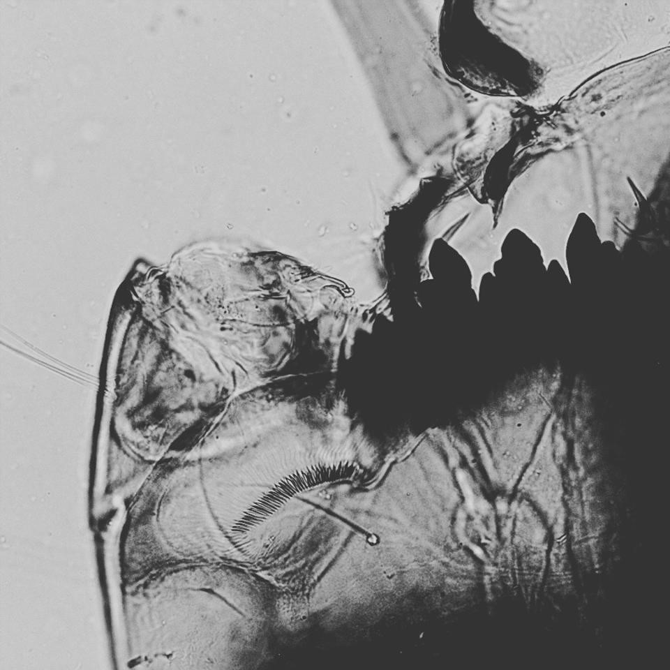
Featured image: a modern reference photograph of a Chironomus tentans head capsule by ThedimitrijaS, CC BY 4.0, unmodified. It illustrates one evidence type, not a fossil from the invented examples.

This guide connects with The Gold Standard of Education and How X Works: learn the mechanism, test an explanation and use the relationship in a changed setting. All numerical datasets here are invented teaching examples, not reported field measurements.
Find your next question
Choose a route, or read from the beginning. Teaching chapters stay open; the grouped index helps you return to a method or calculation.
Full chapter index · Practice and answers · Connected guides and sources
Chapter index
Understand the ecological question · Chapters 1–3
Build time and context · Chapters 4–6
Compare communities · Chapters 7–10
Test explanations · Chapters 11–13
Practise and continue · Chapters 14–16
CHAPTER 1 OF 16 · Understand the ecological question
1. Past ecology begins with a relationship to explain
An environmental reconstruction becomes clearer when the question names both a biological pattern and a possible process. Did aquatic communities change as a lake became shallower? Did woodland composition shift alongside a change in disturbance? These are more testable than asking what the entire past landscape was like.
Identify the geographical area, interval and ecological relationship of interest. A local wetland question may need a different archive from a regional vegetation question. A single basin cannot automatically represent a whole country.
The useful starting point is an observation that could change your mind. Specify which biological remains, sediment features or independently dated evidence would support one explanation over another. That makes the investigation an inquiry rather than an illustrated story.
CHAPTER 2 OF 16 · Understand the ecological question
2. A preserved assemblage is not the original living community
An assemblage is a set of remains recovered under a defined method. Its composition depends on biological production, transport, deposition, survival and recovery. Organisms that lived together need not be preserved in the same proportions.
Durable structures may accumulate while delicate tissues disappear. Water can carry remains away from their original habitat. A sample may mix locally produced material with particles arriving from a much wider area.
Describe the recovered evidence before reconstructing the community. If the method retains only one size fraction or one fossil group, make that boundary visible. The missing organisms are part of the uncertainty, rather than evidence that they never existed.
CHAPTER 3 OF 16 · Understand the ecological question
3. Match the archive to the spatial scale
Pollen, plant macroremains and aquatic microfossils can have different source areas. Their occurrence in one sediment interval does not mean they all describe the same square metre of habitat. Source scale is part of proxy interpretation.
A shoreline plant fragment may give comparatively local evidence, while some pollen can travel farther. The pattern depends on the organism and setting. Lake size, inflows and surrounding vegetation influence how material reaches the archive.
Choose a claim that fits the evidence coverage. A statement about changing inputs to one basin may be well supported even when a regional forest-cover estimate is not. Increasing the precision of a count does not automatically increase its geographical representativeness.
CHAPTER 4 OF 16 · Build time and context
4. Sediment formation shapes the sequence before analysis begins
Sediment is deposited through processes that can vary over time. Changes in inflow, erosion, lake level or biological production can alter accumulation. Mixing, erosion surfaces and interruptions can disrupt a simple depth sequence.
Log lithology and structures alongside biological samples. A sudden change in fossil concentration across a sandy layer may require a sediment-supply explanation before an ecological one. An event deposit can compress or mix material that accumulated over different times.
Stratigraphic context allows these alternatives to be tested. Preserve the relationship between samples, photographs and core descriptions. A microscope result without its depositional setting can be accurate as an identification yet weak as a history.
CHAPTER 5 OF 16 · Build time and context
5. An age model is an inference with uncertainty
Depth indicates position in a sequence; age requires additional evidence. Suitable dated horizons and an explicit model connect the two. Accumulation may be irregular, and not every layer has a direct date.
Radiocarbon dating requires appropriate material selection and calibration. Older material redeposited into a younger layer can complicate the estimate. Other dating techniques answer different questions and have their own requirements.
Carry age uncertainty into the ecological interpretation. If a transition’s age range overlaps several proposed events, do not select a unique cause merely because one event has a memorable name. The chronology must discriminate at the scale of the claim.
CHAPTER 6 OF 16 · Build time and context
6. Calculate the time represented by a sample
In an invented interval, sediment accumulates at 0.05 cm per year. A 1 cm-thick sample represents approximately 1/0.05 = 20 years under a constant-rate model. A 2 cm sample represents roughly 40 years.
At a slower rate of 0.01 cm per year, the same 1 cm sample represents 100 years. Equal sample thickness does not guarantee equal time resolution, even within one core.
This arithmetic is conditional on the model. Mixing or an event deposit can make the effective time window more complicated. Sampling every centimetre does not by itself establish annual resolution or permit the reconstruction of a short event.
| Invented accumulation rate | Sample thickness | Approximate time span |
|---|---|---|
| 0.05 cm/year | 1 cm | 20 years |
| 0.05 cm/year | 2 cm | 40 years |
| 0.01 cm/year | 1 cm | 100 years |
CHAPTER 7 OF 16 · Compare communities
7. Choose the quantity before comparing communities
Counts, proportions, concentrations and accumulation rates answer different questions. A count depends on counting effort; a proportion has a shared denominator; concentration includes sediment quantity; an accumulation rate also requires time.
Comparable methods matter. If one sample has twice the counted effort, raw totals can differ without any ecological change. If one laboratory excludes an unidentified category, its percentages may not share another laboratory’s denominator.
Set out the unit, taxonomic resolution and exclusions before interpreting a chart. Comparisons become more useful when another analyst can reconstruct exactly what entered each number.
Two invented samples each contain 100 identified remains in three ecological groups. Sample A contains 60, 30 and 10; Sample B contains 20, 50 and 30. Group 1 falls from 60% to 20%, while the other groups gain relative share.
A simple Bray–Curtis dissimilarity is the sum of absolute differences divided by the sum of the two sample totals. Here the differences are 40, 20 and 20: D = 80/200 = 0.40.
The value quantifies a difference under this definition. It is not a 40% temperature change, a 40% loss of habitat or proof of a particular mechanism. Equal counting totals make the composition comparison straightforward; unequal effort needs an appropriate comparison strategy.
| Invented ecological group | Sample A | Sample B | Absolute difference |
|---|---|---|---|
| 1 | 60 | 20 | 40 |
| 2 | 30 | 50 | 20 |
| 3 | 10 | 30 | 20 |
| Total | 100 | 100 | 80 |
CHAPTER 9 OF 16 · Compare communities
9. An index summarises difference without identifying its cause
A dissimilarity value compresses information. Two comparisons can have the same value while involving different groups and ecological directions. Inspect the taxon-level pattern alongside the summary.
Bray–Curtis also depends on the chosen data representation. Raw counts can reflect total abundance or sampling effort; proportions emphasise composition. A value calculated from one representation should not silently inherit the meaning of another.
Use the index to locate and describe change, then investigate why the change occurred. The University of Maryland worked analysis distinguishes similarity from its complementary dissimilarity, a useful reminder to label both the formula and the direction of the scale.
CHAPTER 10 OF 16 · Compare communities
10. Preservation can imitate ecological turnover
Suppose an invented deposit originally contains equal numbers of two groups. If one survives burial and processing more readily, its recovered share rises even when the living community never changed. This is an alternative mechanism for the observed pattern.
Inspect fragmentation, surface condition, dissolution and consistency across independently prepared material. A preservation change may be associated with a sedimentary transition, so it can appear exactly where an ecological event is being proposed.
Assessing taphonomy does not make the fossil record unusable. It identifies which relationships are dependable and where a stronger conclusion needs additional evidence. A transparent partial reconstruction is better than an untested complete landscape.
CHAPTER 11 OF 16 · Test explanations
11. Multiple proxies help when their sensitivities are understood
Pollen can inform vegetation inputs; chironomid remains can support calibrated questions about lake conditions; diatoms can contribute aquatic ecological evidence. Their responses overlap, but they are not interchangeable.
Agreement is strongest when the proposed mechanism predicts the response of each proxy. A shared shift might instead reflect one common depositional process affecting all material. Several indicators are not automatically several independent tests.
Compare timing, source area, preservation and ecological sensitivity. If proxies disagree, investigate the discrepancy rather than averaging it away. Different seasons, habitats or response lags may explain why the indicators carry different signals.
CHAPTER 12 OF 16 · Test explanations
12. Separate climate, disturbance and human activity
A shift towards open-ground vegetation can be compatible with climate change, fire, altered water levels, clearance or a changing pollen source area. A plausible cause is not yet an identified cause.
List the evidence that would discriminate between alternatives. A land-use explanation may benefit from archaeological information with suitable chronology; a hydrological explanation may require sediment and aquatic indicators. Charcoal alone does not identify the person or ignition process.
Write the conclusion at the strength the evidence supports. It may establish a community transition and favour one explanation while leaving another unresolved. This is a usable scientific result because its conditions are clear.
CHAPTER 13 OF 16 · Test explanations
13. Past baselines can inform restoration without prescribing a replica
Historical ecological records can reveal that a recent observed state is not the only state a system has occupied. They can inform questions about vegetation, hydrology, disturbance and persistence over longer intervals than monitoring alone.
Restoration still faces current conditions, ecological feasibility and explicit goals. A past assemblage is evidence about a former system, not an automatic instruction to recreate it exactly under a different climate or land-use setting.
Use palaeoecology to expand the evidence considered. Explain which past functions or relationships are relevant, how confidently they are reconstructed and what contemporary observations are needed before choosing an intervention.
CHAPTER 14 OF 16 · Practise and continue
14. Write a conclusion another investigator can revise
Preserve raw counts, sample context, identification rules, preparation methods and the age model. Report the observed pattern separately from the reconstructed environment and the proposed cause.
State the most important uncertainty and the next discriminating test. For example: assemblage composition changed, the available model places it within a broad interval, and additional dates are needed to compare two proposed drivers.
Students can practise by rewriting a confident headline into three bounded statements. The task is not to remove meaning; it is to make each claim traceable to evidence and identify the observation that would improve it.
CHAPTER 15 OF 16 · Practise and continue
15. Practice composition and time-window reasoning
Use the invented values below independently. Begin with the quantity being asked for, show the arithmetic and finish with an interpretation that stays within its unit and assumptions.
After checking, explain why a numerical difference cannot by itself select an ecological cause. This is the relationship to carry into an unfamiliar fossil dataset.
Try it independently
Samples A = [50, 30, 20] and B = [30, 30, 40] each total 100. Calculate Bray–Curtis dissimilarity.
A 1.5 cm interval accumulated at 0.03 cm/year under a constant-rate model. What is its approximate time window?
Two proxies change within a broadly dated century. Does this establish that one short historical event caused both changes?
Show answers and reasoning
Absolute differences total 20 + 0 + 20 = 40; D = 40/200 = 0.20.
1.5/0.03 = 50 years, conditional on the model and without additional mixing.
No. Examine age uncertainty, proxy sensitivities, deposition and competing mechanisms. Shared timing at coarse resolution is insufficient for unique attribution.
CHAPTER 16 OF 16 · Practise and continue
16. Follow the palaeoecology learning directory
Use Palynology for pollen production, concentration and influx; Micropalaeontology for fossil groups and recovery; and Stratigraphy for sequence relationships.
Continue into Chironomid Palaeoecology, Testate Amoebae Analysis and Palaeobotany for specialist evidence.
Primary-method reading includes the lake-sediment uncertainty workshop report, NOAA’s palaeoclimate archive, and the University of Maryland assemblage-comparison example. These support the methods; all counts and time-window calculations in this guide are original illustrations.
Contents · Previous chapter · The Gold Standard master hub · Continue with How X Works