
EDUKATE · THE GOLD STANDARD
Find your next learning step
Choose the question your image needs to answer. Follow a route through image formation, instrument choice, measurement or interpretation, then test whether the evidence supports the claim.
Full chapter index · Diagnose the difficulty · Specialist reading library · Science Learning Hub
Microscopy uses instruments to investigate structures and processes that are difficult or impossible to examine with the unaided eye. Depending on the method, an image may be formed from transmitted light, fluorescence, electron signals or a probe’s interaction with a surface. The image is evidence produced by a measurement process, not an unfiltered miniature view of reality.
The gold standard is being able to explain what generated the contrast, how spatial scale was established, what detail the instrument could resolve and which conclusions remain uncertain. A sharp, colourful image can still have an incorrect scale bar, an unrepresentative field of view or an unsupported interpretation. Good microscopy joins useful images to checkable reasoning.
This root connects Optics, Physics, Cell Biology, Microbiology and Materials. It organises the specialist articles already in the ecosystem rather than treating every method as a separate subject to learn from scratch. Start with the mechanism your question requires, then follow the corresponding reading path.
The educational aim follows The Gold Standard of Education: learning that transfers into life. Use the proportional reasoning and careful explanation developed through the Secondary 1 Mathematics learning page to check units, ratios and measurements. Numerical examples below are invented teaching cases, not measurements from the featured photograph or a research experiment.
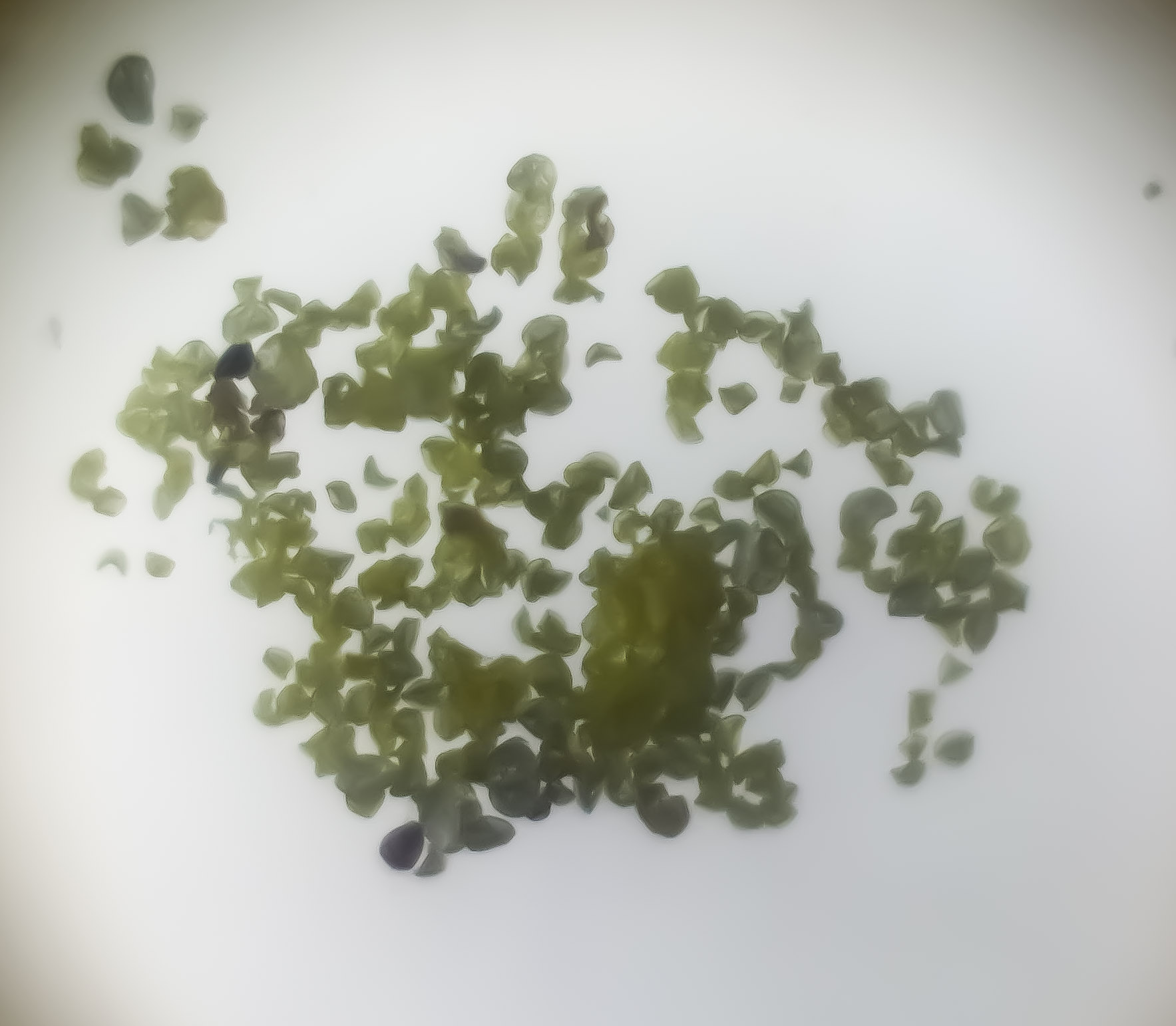
Featured photograph: modern pollen under the microscope, by Korinna, via Wikimedia Commons, licensed CC BY 4.0. Reused without intentional modification to the source image; the site may resize it for display. It is an illustration of microscopy, not evidence for the calculations below.

Full chapter index
Understand the image · Chapters 1–5
Choose the signal · Chapters 6–10
Prepare and measure · Chapters 11–14
Check the evidence · Chapters 15–18
Diagnose and transfer · Chapters 19–22
CHAPTER 1 OF 22 · Understand the image
1. Start with the question, not the highest magnification
Before selecting an instrument, decide what you need to learn. Counting cells, measuring a surface step, locating a labelled protein and distinguishing crystalline orientations are different tasks. They require different signals, preparation and analysis. An instrument that produces a beautiful picture may not measure the quantity your question asks about.
Write the intended observation and inference separately. “There are several bright spots in this field” describes an image. “This treatment increased the amount of a particular protein” is a stronger claim requiring suitable labelling, acquisition controls, independent samples and a measurement strategy. The second statement cannot be justified merely by repeating the first more confidently.
Also specify the scale and whether change over time matters. A wide field may be needed for distribution, while a small field can reveal fine structure. A process that changes rapidly may be poorly represented by a long acquisition. Improving one dimension of performance can cost something elsewhere.
For a first exercise, take a published microscopy figure with an explanatory caption. Identify the specimen, imaging method, visible scale and actual question. Then write one thing the image alone cannot establish. This small habit makes later technical choices easier to understand.
In transmitted-light microscopy, illumination passes through a specimen before reaching the imaging system. Variations in absorption, scattering or optical phase can contribute to contrast, depending on the method. In fluorescence microscopy, a suitable fluorophore is excited and its emitted light is detected. These signals answer related but not identical questions.
An electron microscope uses electrons and detectors rather than an ordinary optical photograph of the specimen. A scanning probe instrument records an interaction between a small probe and a surface. The resulting map may be displayed with shading or colour, but that display is not necessarily the specimen’s natural appearance.
Trace the chain in words: specimen interaction, collection, detection, numerical representation and display. At each stage, ask what could change the result. The same specimen can look different under different contrast methods because each method emphasises a different property.
Use Microscopes, Cells and Seeing Scale as a starting application, then connect to How Science Works | Optics. The transferable point is not to memorise an instrument catalogue. It is to identify the measured signal before naming the structure you think it represents.
CHAPTER 3 OF 22 · Understand the image
3. Magnification makes an image larger; resolution separates detail
Magnification is a size ratio. In a simple visual compound microscope with a 10× eyepiece and a 40× objective, nominal total magnification is 10 × 40 = 400×. This is an optical viewing calculation, not a reliable label for every digital display of the resulting image.
Resolution concerns the ability to distinguish nearby features. Enlarging a blurred image does not necessarily separate two points that the original imaging system merged. Increasing display size can make the existing information easier to inspect while adding no newly measured detail. This is why a very large magnification number is not a sufficient statement of performance.
Digital magnification also depends on the displayed image size. The same file may appear small on a phone and large on a projection screen. A properly constructed scale bar travels with the image geometry and is more useful than a claim such as “400×” detached from the viewing conditions.
Try explaining a familiar photograph enlarged beyond its useful detail. Then return to microscopy and distinguish the lens magnification, the sampled image and the final display. If those three stages are clear, the calibration examples in Chapter 12 become much less mysterious.
CHAPTER 4 OF 22 · Understand the image
4. Resolution has a physical model and practical limits
For an idealised diffraction-limited optical system under a Rayleigh-type lateral resolution criterion, a commonly used estimate is d ≈ 0.61λ/NA. Here d is a separation distance, λ is the wavelength and NA is the objective’s numerical aperture. The coefficient and applicability depend on the resolution criterion and imaging conditions; this is not a universal formula for every microscopy method.
Take an invented comparison using λ = 550 nm and NA = 0.65. The estimate is 0.61 × 550 / 0.65 ≈ 516 nm, or 0.516 µm. If NA is 1.30 at the same wavelength, the estimate becomes about 258 nm, or 0.258 µm. A smaller d means closer features can potentially be distinguished.
These are theoretical estimates, not certified performance figures for a particular microscope. Aberrations, alignment, specimen contrast, motion, sampling and noise may prevent the practical image from achieving them. Resolving detail along the optical axis also differs from resolving it laterally.
Nikon’s resolution explanation provides the optical context. When reporting a result, state the relevant method and conditions rather than treating the calculation as proof that every feature of that size is visible.
CHAPTER 5 OF 22 · Understand the image
5. Numerical aperture, collection and working conditions
Numerical aperture is defined as NA = n sin θ, where n is the refractive index of the medium between specimen and objective and θ is the half-angle of the accepted light cone. It describes collection geometry and contributes to resolving performance. It is not the same quantity as magnification.
Two objectives with the same nominal magnification can have different numerical apertures, corrections and working conditions. Their images need not contain the same level of useful detail. Read the markings and instrument documentation rather than assuming that changing magnification alone defines the optical setup.
Immersion objectives are designed for particular media and conditions. Using the wrong medium, coverslip or preparation can introduce problems rather than improve the image. Follow the manufacturer’s guidance and trained supervision; immersion is not a general instruction to add a liquid to any lens.
Before comparing images, record the objective, numerical aperture, medium and relevant acquisition settings. Nikon’s Numerical Aperture resource explains the geometry. The learning checkpoint is being able to say why a different collection cone can change the information captured even when the displayed image size stays similar.
An unstained transparent specimen can be difficult to see even when the optics could resolve its dimensions. Contrast determines whether differences produce a detectable signal against their surroundings. Bright-field images often show structures through differences in transmitted intensity; staining can increase visibility but also changes the preparation.
Phase contrast converts differences in optical phase into differences of image intensity. It can reveal transparent structures without requiring the same staining approach as conventional stained bright-field work. Its characteristic image features, including possible halos, must be interpreted as part of the method rather than automatically treated as specimen boundaries.
Polarised-light techniques can reveal how a specimen changes the polarisation of light. Their usefulness in mineral and material work comes from optical properties, orientation and preparation, not simply from producing striking colours. Colour appearance alone is not a complete mineral identification.
Read Nikon’s Phase Contrast overview, then connect the application to Mineralogy or Metallurgy. Ask what property is responsible for the contrast and whether a different preparation would alter it.
CHAPTER 7 OF 22 · Choose the signal
7. Fluorescence: a labelled signal needs controls
Fluorescence microscopy detects emitted light from suitable fluorophores following excitation. Filters and other optical components help separate desired emission from excitation and unwanted signals. A fluorescent image may reveal the distribution of a label rather than all structures present in the specimen.
Interpretation therefore depends on the label. If an antibody-associated signal appears in a region, that observation does not by itself establish perfect specificity. Background, autofluorescence, channel cross-talk and non-specific binding can affect what is seen. Controls should address the relevant uncertainty rather than appear as a ritual checklist.
Photobleaching means that fluorescence can decline during illumination. A change in signal over time can therefore reflect acquisition history as well as the process being studied. Exposure and illumination must be considered when comparing images. Brightness on a screen is not a direct molecular count.
Begin with Immunofluorescence Microscopy and Nikon’s Fluorescence resources. Continue into Molecular Biology when the question concerns a labelled molecular target. Keep the claim proportional to the validation of the signal.
CHAPTER 8 OF 22 · Choose the signal
8. Optical sectioning and super-resolution are different advances
Confocal microscopy uses an arrangement that rejects much out-of-focus light, enabling optical sectioning. A series of sections can support a three-dimensional representation, but section spacing, axial resolution, signal quality and reconstruction choices still matter. An attractive rotating reconstruction is not automatically a complete or distortion-free object.
Light-sheet and two-photon approaches offer different illumination and detection strategies for particular specimens and questions. They are not simply interchangeable labels for “better microscopy.” The trade-offs include specimen access, imaging depth, speed, light exposure and the kind of information required.
Super-resolution methods can recover spatial information beyond conventional diffraction-limited imaging through specific physical and computational strategies. Localising an isolated emitter precisely is not the same as resolving a densely labelled structure with equal precision everywhere. Labelling density, motion and reconstruction assumptions remain important.
Use Confocal Microscopy, Light-Sheet Fluorescence Microscopy and Two-Photon Excitation Microscopy for the first branches. The super-resolution reading paths in Chapter 18 distinguish methods rather than collapsing them into one promised resolution number. Nikon’s Confocal and Super-Resolution overviews provide external orientation.
CHAPTER 9 OF 22 · Choose the signal
9. SEM and TEM collect different electron evidence
Scanning electron microscopy, or SEM, commonly scans a focused electron beam across a specimen and builds images from detected signals such as secondary or backscattered electrons. Which detector is used affects the contrast. A surface-like appearance does not mean that every bright region has the same physical explanation.
Transmission electron microscopy, or TEM, uses electrons transmitted through a suitably prepared specimen. It can provide evidence about internal structure and diffraction under appropriate conditions. A sufficiently electron-transparent specimen is important; “put the same sample in a stronger microscope” is not an adequate preparation plan.
Electron images do not ordinarily record natural optical colour. Colours added for explanation or to represent different measured channels must be described. Preparation, charging, beam damage and contamination can affect interpretation. Relevant instrument and specimen conditions should accompany the image.
Continue through Scanning Electron Microscopy, Transmission Electron Microscopy and Cryo-Electron Microscopy. JEOL’s SEM–TEM comparison explains the detector distinction. Cryogenic preparation is a specialised approach, not permission to assume that every image shows an untouched living specimen.
CHAPTER 10 OF 22 · Choose the signal
10. Scanning probes map an interaction with a surface
Atomic force microscopy, or AFM, uses a small probe associated with a cantilever to investigate a surface. Depending on the mode, measured interactions can support topographic or mechanical information. The output is a measured map with a particular interaction model, not an ordinary close-up photograph.
Probe geometry can affect apparent feature shape. A finite-sized tip does not reach every narrow recess or trace every steep feature without limitations. Calibration of dimensions and interaction measurements matters. An impressive height map still needs a record of how the result was acquired and interpreted.
Scanning tunnelling microscopy, or STM, measures a tunnelling-current interaction between a tip and a suitable surface under controlled conditions. Its contrast is sensitive to electronic properties as well as geometry. Reading every bright feature as a literal ball-shaped atom would miss the measurement mechanism.
Follow Atomic Force Microscopy and Scanning Tunnelling Microscopy, then connect to Nanotechnology. NIST’s scanning probe calibration work and STM introduction provide primary technical context.
A specimen may be sectioned, fixed, stained, mounted, polished, coated or otherwise prepared before imaging. Each step makes some observations possible and may alter other properties. A preparation record is therefore part of the explanation, not merely a list of laboratory chores placed before the real science.
For a teaching comparison, imagine two sections cut through the same kind of three-dimensional object at different orientations. Their profiles can look different without the underlying objects having different identities. Thickness, cutting angle and deformation may influence what appears to be a change in shape.
An artefact is a feature introduced or substantially affected by the preparation or measurement process rather than a faithful representation of the property being investigated. Repeating the same preparation can repeat the same artefact. A second method or an appropriate control may be needed to distinguish the possibilities.
Use approved prepared slides or supervised teaching materials for introductory work. This article is not a protocol for handling biological hazards, chemicals, lasers, vacuum equipment or electron microscopes. Specialised preparation requires relevant training and local procedures. Connect tissue interpretation to Histology and material preparation to Materials.
CHAPTER 12 OF 22 · Prepare and measure
12. Calibrate pixels, then protect the scale bar
Spatial calibration connects image distances to specimen distances. Suppose a suitable reference shows that 100 µm spans 400 acquisition pixels. The scale is 100/400 = 0.25 µm per pixel. A feature spanning 120 pixels would measure 120 × 0.25 = 30 µm along the measured direction, subject to the calibration and boundary uncertainty.
A bar labelled 20 µm must span 20/0.25 = 80 pixels in that original image. If the image is resampled to half its original width and height, the same feature spans 60 output pixels while still representing 30 µm. The new spatial scale is 0.50 µm per output pixel, and a newly drawn 20 µm bar should span 40 output pixels.
| Quantity | Original image | Half-width, half-height output |
|---|---|---|
| Spatial scale | 0.25 µm/pixel | 0.50 µm/pixel |
| 30 µm feature | 120 pixels | 60 pixels |
| Correct 20 µm bar | 80 pixels | 40 pixels |
If an existing embedded bar is uniformly resized together with the image, their geometrical relationship is retained. Drawing a new bar afterwards requires the corresponding output calibration. Cropping without resampling is a different operation: removing surrounding pixels does not by itself change the physical size represented by each retained pixel.
Read How to Calculate Actual Size from a Microscope Image and the fictional Case 147: a scale bar becomes twice too long for further practice. ImageJ spatial calibration and the Office of Research Integrity guidance on magnification explain why calibration must survive the final figure.
CHAPTER 13 OF 22 · Prepare and measure
13. Sampling and field of view limit what is recorded
Optical resolution and digital sampling are distinct. A sensor must sample the image finely enough to capture relevant spatial information. Having many pixels does not repair an optical system that never separated the features, while coarse sampling can lose detail that the optics could have conveyed.
For a simple periodic test pattern with a 1 µm spatial period, the Nyquist minimum corresponds to a sampling interval of 0.5 µm or smaller. This idealised frequency example is not a universal promise that any two-pixel object will be accurately resolved or measured. Practical microscopy may require finer sampling for the method and analysis.
Consider another invented image with 2,048 pixels across and a calibrated scale of 0.20 µm per pixel. Its field width is 2,048 × 0.20 = 409.6 µm. A central crop 1,024 pixels wide, without resampling, covers 204.8 µm and retains the same pixel scale. Enlarging that crop for display does not turn it into an observation of a wider field.
Nikon’s Nyquist sampling explanation provides the frequency context. Always distinguish specimen field of view, acquisition pixel spacing and output dimensions. This prevents confusing a file-size change with a physical measurement.
CHAPTER 14 OF 22 · Prepare and measure
14. Intensity, background and saturation answer different questions
A detector records a signal within its operating range. Background and instrument settings can affect numerical values. A bright region may contain more detected signal, but comparison across samples requires suitable controls and compatible acquisition conditions. A display slider can change appearance without changing the original measured values.
In an invented example, one region has mean intensity 140 arbitrary units and a relevant background estimate is 40. The background-corrected mean is 100. Another comparable region has mean 180 with the same background estimate, giving 140. The corrected ratio is 140/100 = 1.4, not the uncorrected 180/140 ≈ 1.29.
That arithmetic assumes the background estimate is suitable and the measurements are comparable. It does not establish that there is exactly 40% more protein. Label efficiency, detector response, specimen geometry and other conditions must support the biological interpretation. The calculation is a signal comparison before it is a molecular claim.
Saturation clips values at a detector or encoding limit. A region at the maximum recorded value may have lost information about how much brighter it truly was. Adjusting the display afterwards cannot recover the missing measurement. The Microscopy for Beginners intensity guide discusses why these comparisons require care.
CHAPTER 15 OF 22 · Check the evidence
15. Segmentation is an analytical decision, not a discovered boundary
Segmentation assigns pixels or voxels to objects or regions for analysis. A threshold, a trained model or another algorithm can turn a grey-level image into a set of counted objects. The result depends on the rule, image quality and the property the rule was designed to detect.
If two touching cells are counted as one, the estimated number falls and the apparent average object size can rise. If noise is counted as small objects, the number can rise. A numerical output with many decimal places does not reveal whether these assignments were correct.
Test the method on representative examples, including difficult cases. Compare masks with the underlying images and use an independent check suitable for the task. Set the analysis plan without tuning each group towards a preferred conclusion. If different conditions need different treatment, justify and document the choice.
Artificial intelligence can help identify patterns but can also fail on unfamiliar preparations or imaging settings. Preserve the original data, analysis version and relevant parameters. The question is whether the measured quantity is valid for the intended use, not whether the software is sophisticated. Connect uncertainty and comparison to Statistics.
CHAPTER 16 OF 22 · Check the evidence
16. A field of view is not an independent experiment
A hundred cells from one dish do not automatically provide a hundred independent biological replicates. Cells can share the same preparation, treatment environment and batch effects. The appropriate unit of replication depends on how the experiment was designed and what population the claim concerns.
Suppose a fictional study images five fields from each of three independently prepared specimens in each group. The fields provide within-specimen information. They do not erase the specimen structure and create fifteen independent specimen preparations. Analysis should respect this hierarchy rather than inflate confidence by relabelling observations.
Field selection matters too. Choosing only the cleanest or most dramatic image can misrepresent the distribution. A consistent sampling rule, documented exclusions and suitable blinding can reduce selection bias. Report both the number of independent units and the number of observations within them.
Use Statistics to understand the distinction between more observations and more independent information. A microscopy image can be excellent evidence that a feature exists in that field while remaining weak evidence about how common the feature is across a larger population.
CHAPTER 17 OF 22 · Check the evidence
17. Make the claim no stronger than the imaging chain
Separate three levels: what was recorded, what it was measured to be and what you infer from it. A bright spot, a measured distribution of labelled spots and a conclusion about a biological process are different statements. Each transition needs assumptions and evidence.
Colocalisation at the scale of an image does not by itself prove direct molecular binding. A projection can place objects on top of one another even when their positions differ along depth. Likewise, a surface feature in one view does not reveal every internal property of the material.
Preserve raw data and use analysis copies with documented transformations. For presentation, label channels, scale, sections or projections and relevant processing. Make comparisons readable without hiding information. Showing separate greyscale channels as well as a composite can help readers inspect what each signal contributes.
The image-presentation guide explains responsible figure handling. For reusable evidence, read BioImage Archive and Reusable Image Evidence and visit the EMBL-EBI BioImage Archive. The dataset, metadata and analysis history often answer questions that a small published panel cannot.
CHAPTER 18 OF 22 · Check the evidence
18. Specialist reading library: follow the mechanism
Begin with scale and the subject
Use Microscopes, Cells and Seeing Scale, Actual Size from a Microscope Image and Case 147: the resized scale bar for the foundations. Continue into Optics, Measurement and Science Learning Hub. For the specimen context, choose Cell Biology, Microbiology, Molecular Biology, Mineralogy or Metallurgy.
Locate signals and follow changing processes
Choose Immunofluorescence for antibody-associated spatial signals; Confocal, Light-Sheet and Two-Photon Microscopy for different optical acquisition strategies. Total Internal Reflection Fluorescence develops the near-surface branch. Fluorescence Lifetime Imaging, Fluorescence Recovery After Photobleaching and Fluorescence Correlation Spectroscopy organise different questions about fluorescence behaviour. They do not all measure the same property.
Go beyond conventional optical detail
Follow Structured Illumination, Stimulated Emission Depletion, Photoactivated Localization, Stochastic Optical Reconstruction, MINFLUX and Expansion Microscopy as distinct specialist reading paths. Compare the evidence and assumptions described in each article rather than choosing a method by its smallest advertised number.
Examine surfaces, interiors and correlated evidence
Use SEM, TEM, Cryo-Electron Microscopy and Cryo-Electron Tomography for the electron-imaging branches. Continue into Electron Backscatter Diffraction for grain-orientation evidence. Correlative Light and Electron Microscopy connects modalities; AFM and STM develop the scanning-probe branches.
Extend the kinds of interaction studied
The ecosystem also contains Scanning Near-Field Optical Microscopy, Second-Harmonic Generation Microscopy, Brillouin Microscopy and Photoacoustic Microscopy. Start each by identifying its measured signal, not by assuming that every displayed map is an ordinary photograph.
Return to preparation, context and reuse
Connect Histology, Ceramic Petrography, Soil Micromorphology and Palynology to the specimen-specific questions they address. Use BioImage Archive and Reusable Image Evidence for data reuse and Reporting a Research Microscope Malfunction for precise technical communication. Materials, Nanotechnology and Statistics supply wider interpretation routes.
CHAPTER 19 OF 22 · Diagnose and transfer
19. Diagnose the bottleneck before changing instruments
If the image is larger but no more informative, separate magnification from resolution. Revisit Chapters 3–5 and identify what limited the information: optics, contrast, sampling, motion or noise. Buying or selecting a higher magnification is not an explanation of the bottleneck.
If a structure is visible but its measured size changes after export, audit the calibration and transformations. Check the original scale, cropping, resampling and whether the bar was embedded or drawn later. Recalculate one known distance independently. Chapter 12 provides a small test case that should give the same physical length before and after resizing.
If two groups look different only after display adjustment, compare the acquisition conditions and raw numerical ranges. Look for saturation, incompatible exposure, background variation or a presentation choice that exaggerates a difference. A useful repair addresses the source of uncertainty rather than making the picture more persuasive.
If counts or areas change dramatically when an analysis setting is altered, inspect the segmentation masks and representative difficult cases. If an apparently strong finding rests on many fields from one preparation, revisit replication. More images do not automatically repair a missing independent comparison.
Finish by naming one observation, one supported inference and one unresolved alternative explanation. If those cannot be separated, the next step is usually better documentation, a suitable control or a narrower claim—not simply a more confident caption.
Can a microscope see anything if the magnification is high enough?
No. Magnification, resolution, contrast, specimen preparation and signal quality are different constraints. Enlarging a recorded image cannot guarantee new measured detail. The method must interact with the property being investigated in a useful and interpretable way.
Are all colours in microscopy natural colours?
No. Colour may represent optical appearance, a selected fluorescence channel, a measured quantity or an explanatory assignment. Read the caption and legend. An assigned colour can communicate valid data, but it should not be mistaken for an unprocessed natural-colour view.
Is a scale bar better than a magnification label?
A correctly calibrated bar usually communicates specimen scale more robustly across display sizes because it is part of the image geometry. It can still be wrong if constructed or transformed incorrectly. Chapter 12 shows why the final exported figure must be checked.
Does a bright fluorescent spot prove a particular molecule is present?
Not by itself. The inference depends on the label, controls, background and measurement conditions. A fluorescent signal is an observation; its molecular interpretation needs additional justification. This article is educational and does not support diagnosis from a specimen image.
Is every cell in one image a separate replicate?
No. The experimental unit depends on how independent preparations and treatments were created. Cells and fields can be nested within a shared specimen. Report that structure and use analysis appropriate to the question.
Can software restore all lost detail?
No. Reconstruction and restoration can be useful under explicit assumptions, but a visually plausible output is not proof that all displayed detail was independently observed. Preserve originals, validate the method and disclose relevant processing.
Must beginners use advanced instruments?
No. Prepared educational images and supervised light microscopy can teach scale, observation, calibration and uncertainty. Those reasoning skills remain necessary when the instrument becomes more sophisticated.
CHAPTER 21 OF 22 · Diagnose and transfer
21. A four-week route to transferable understanding
In week one, annotate three existing educational images. For each, identify the specimen, signal, scale and question. Write what is directly visible before writing an interpretation. Choose examples from different methods so the exercise does not become a habit of recognising only one visual style.
In week two, practise measurement with supplied calibrated images or invented data. Reconstruct Chapter 12 without looking. Then change the reference to 50 µm spanning 200 pixels: the scale remains 0.25 µm per pixel. A 36-pixel feature represents 9 µm. Explain why the unit conversion, not the apparent screen size, determines the answer.
In week three, compare two possible methods for one question. Decide what property each measures, what preparation is required and what limitation matters most. Use Chapter 18 to locate the closest specialist branch. The aim is a justified choice, not a declaration that one instrument is universally best.
In week four, write a short figure explanation using a public educational dataset with its accompanying metadata. Include a calibrated scale where available, a precise observation, a supported inference and one limitation. Do not invent missing settings or reconstruct scale from a feature whose true dimensions are unknown.
Test transfer by asking another reader to explain what your figure establishes. If they infer more than the data support, revise the caption or presentation. The completion standard is being able to defend the chain from specimen to claim while remaining clear about uncertainty.
This is an educational root for understanding microscopy and connecting specialist reading. It is not an instrument operating manual, a biological identification service, a clinical interpretation guide or a substitute for laboratory training. All worked numbers are hypothetical and independent of the featured image.
Nikon MicroscopyU: Resolution and Numerical Aperture explain the optical foundations. Its Phase Contrast, Fluorescence, Confocal and Super-Resolution resources extend the method map.
JEOL: TEM versus SEM explains the electron-imaging distinction. NIST: Scanning Probe Microscopy Calibrations and Standards and its STM introduction provide primary context for probe measurements.
ImageJ: Spatial Calibration and Office of Research Integrity: Issues with Magnification support careful scale reporting. The Nikon sampling glossary explains the idealised spatial-frequency example.
For quantitative study, use the Microscopy for Beginners reference guide, including its intensity measurements and image presentation sections. Senft, Diaz-Rohrer and colleagues’ guide to planning quantitative bioimaging experiments provides a broader research framework. The EMBL-EBI BioImage Archive supplies an established route to reusable biological image data.
The standard to keep is simple: identify the signal, preserve the scale, check the analysis and limit the claim to the evidence. Microscopy becomes more than seeing small things when the learner can explain why an image is informative, where it can mislead and what observation would resolve the remaining uncertainty.
Contents · Previous chapter · Learning that transfers into life