
Archaeological chironomid analysis examines the head capsules of non-biting midge larvae preserved in lake sediments to reconstruct environmental change. Identifying these fossil mouthparts can reveal shifts in aquatic communities, and carefully validated modern calibration may support estimates of past summer air temperature. But a chironomid capsule is not an exact thermometer: oxygen, nutrients, lake depth, habitat and sampling can also shape its fossil record.
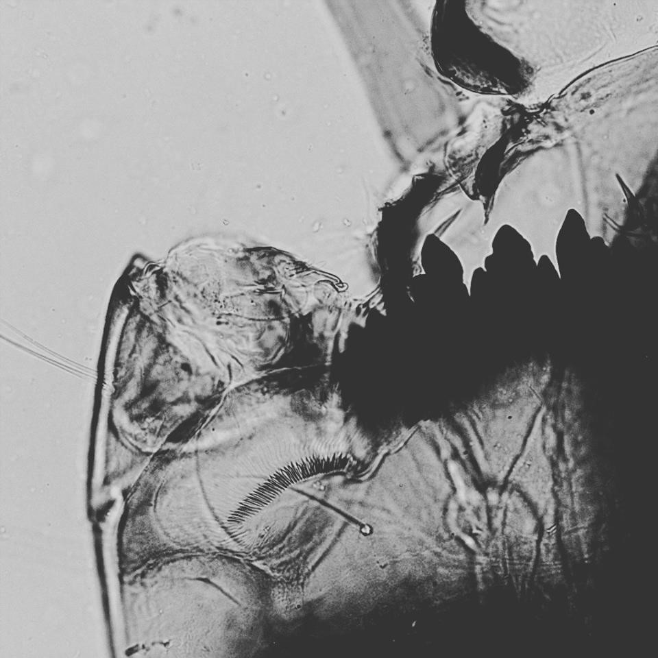
This Gold Standard teaching reference develops the method from first principles—larval anatomy, mentum morphology, taxonomic identification, head-capsule counts, environmental confounders, transfer functions, calibration and uncertainty. An original fictional Pinewater Lake dataset demonstrates the arithmetic without pretending to be excavated evidence. The featured microscope photograph is a genuine modern Chironomus tentans larval head capsule, not a fossil from Pinewater.
For current scientific calibration, see the 2025 study of 182 lakes in eastern North America and a review of chironomid temperature ecology. Both show why modern observations are needed before fossil assemblages become defensible climate estimates.


1. Begin with an observation, not an ancient thermometer
Chironomids are non-biting midges whose larval head capsules often survive in lake sediment. Researchers identify the preserved mouthpart structures and compare fossil assemblages with living or recent communities to infer past aquatic conditions. In suitable regions, empirically calibrated assemblages can be used to reconstruct mean summer air temperature, but the capsule is not itself a thermometer. Its taxon may also respond to lake oxygen, nutrients, substrate, depth and changes in habitat.
Begin a lesson by contrasting three claims. A sediment sample contains a chironomid larval head capsule. The community differs between two depths. A named settlement experienced an unusually hot summer in an exact year. Only the first is directly visible in the microscope; the latter claims require increasingly demanding calibration, chronology and independent context. The standard is to teach the ladder between an identified biological remain and an environmental or historical explanation.
2. Understand the living insect and its aquatic larva
Chironomidae belong to Diptera, the true flies. The adults resemble mosquitoes but are non-biting, while many larvae live in lake and stream sediment, on plants or in other aquatic microhabitats. Larval forms are ecologically diverse and not all chironomids live in deep lakes. Their development, feeding and habitat preferences vary by taxon. This diversity makes them informative as ecological indicators, but it also means a generic ‘midge’ label provides little information.
Give students a life-cycle diagram showing eggs, multiple larval instars, pupa and adult. Ask which life stage produces the durable structures counted in sedimentary palaeoecology. They should draw the larval capsule separately from the whole living organism and understand why an adult midge swarm has a different ecological meaning from a preserved head capsule in a dated lake core.
3. Explain why the head capsule survives
The larval head includes sclerotised parts that can remain recognisable after softer tissues decay. They may preserve mouthparts and structural features useful for identification. Their survival depends on sediment conditions, processing and later disturbance, so a low fossil count need not mean larvae were absent. The object being measured is a preserved head-capsule remain, not a whole animal, a count of adult midges or a direct measure of climate.
Use the credited modern Chironomus tentans head-capsule photograph in this guide. It shows real reference mouthpart anatomy, not a fossil from the invented Pinewater Lake core. Ask students to identify where the mentum and other useful structures would be examined and why the photograph cannot authenticate the fictional numerical exercise. Scientific captions must separate real reference images from hypothetical archaeological data.
4. Learn what a mentum is and why its teeth matter
The mentum is a sclerotised part of the mouth region, and the form, number and arrangement of its teeth can aid identification. Other structures such as ventromental plates, mandibles and antennae can provide additional characters. However, tooth wear, folding, breakage and viewing angle may obscure diagnostic detail. A taxonomic key should not be replaced by the confident recognition of one dark triangular shape.
Assign students two diagrams, one complete and one missing a central mentum tooth. They should record which taxa are plausible and what further structures would be required for more specific identification. A cautious broader morphotype is better than an unjustified species label. The exercise prepares them to build calibration tables whose names reflect the evidence actually available.
5. Treat moulting as a counting problem
Chironomid larvae develop through several instars and shed earlier head capsules as they grow. Fossil sediments may therefore contain multiple capsules produced by different development stages and individuals. A capsule tally is not a one-to-one census of larvae or adult flies. Some capsules may be broken into fragments, while incomplete specimens may be impossible to assign confidently to a specific taxon.
Give students an imaginary collection containing two intact capsules, one partial capsule and several fragments from the same broken head. Ask for separate counts of physical pieces, identifiable capsules and potential duplicate observations. They should keep those units distinct before calculating relative abundance. This basic counting discipline prevents an apparently small mistake from affecting every later temperature reconstruction.
6. Choose a taxonomic resolution the material supports
Chironomid fossil specialists may classify head capsules to genus, species group or distinctive morphotypes, depending on diagnostic structures and regional references. The appropriate resolution varies among groups, and not every fossil can be placed at the same level. A coarse category can combine organisms with differing temperature and lake-environment preferences. Excessive precision, by contrast, can create spurious ecological detail from poorly preserved material.
Ask students to compare how a published temperature model defines its taxa with the categories in their fossil table. If the model distinguishes two morphotypes but the fossil material only supports one broad group, direct substitution may invalidate its assumptions. The lesson should include a rule for uncertain identifications and a discussion of whether multiple categories can be harmonised without discarding crucial ecological differences.
7. Understand that the lake is a mosaic of habitats
Shallow vegetation beds, open-water bottoms, oxygen-rich margins and deeper fine sediments can support different chironomid communities within the same lake. Water depth, temperature, oxygen and substrate can vary together. A central core may receive head capsules from several habitats through normal deposition and water movement. Consequently, an apparent change in warm-associated taxa can reflect shifting habitat availability or lake level as well as climate.
Have learners sketch a lake transect and assign hypothetical chironomid communities to littoral and profundal zones. Ask how falling water levels or expanding vegetation could change the shells recorded at a fixed coring point. Their explanation should keep the source of the fossils spatially separate from the spot where the sediment sample was collected.
8. Explain why oxygen can mimic a temperature change
Dissolved oxygen near the lake bottom may decline when stratification intensifies or when organic matter decomposition consumes oxygen. Some midge larvae tolerate low-oxygen conditions better than others, so communities may shift without a straightforward change in regional air temperature. Warmer water can contribute to stratification but is not the only cause. Nutrient loading, mixing depth, lake morphology and water exchange can also alter oxygen.
Offer students a hypothetical lake whose summer air temperature remains broadly stable while sewage-derived nutrients increase and bottom-water oxygen falls. Ask how larval habitat and fossil head-capsule composition might change. They should recognise the risk that a model trained along a regional temperature gradient can attribute a locally nutrient-driven community shift to apparent warming. Independent oxygen and trophic evidence becomes essential.
9. Consider nutrients, eutrophication and human disturbance
Phosphorus, nitrogen and organic matter inputs can influence algal production, sediment food resources and lake oxygen. Agricultural runoff, wastewater, forestry and natural watershed change can all affect those inputs. Chironomid shifts may therefore be useful for studying environmental impacts, but a temperature transfer function should not automatically be interpreted as an industrial pollution history or vice versa. The same taxon can participate in several ecological responses.
Ask students to compare two claims drawn from an invented settlement pond: ‘the larvae became more tolerant of anoxic conditions’ and ‘summer air temperature rose’. They should list which evidence would support each, including sediment chemistry, diatoms, known land use and instrumental records where available. The exercise teaches that ecological organisms are not single-purpose sensors.
10. Distinguish lake-water temperature from summer air temperature
Larvae experience aquatic conditions, while many calibration models target mean summer or June–August air temperature because a modern regional relationship has been observed between those values and chironomid assemblages. The inferred variable is therefore an empirical statistical target, not an actual thermometer inside the sediment. Lake depth, ice cover, stratification and local hydrology can alter the relation between air and bottom-water temperatures.
Give learners a warm shallow pond and a deeper stratified lake under the same local weather. Ask whether their larvae necessarily inhabit the same thermal environment. They should explain why a calibration result expressed in degrees Celsius of summer air temperature requires a suitable modern reference and ecological checks before being treated as a local water reading.
11. Choose an appropriate modern training set
A transfer function begins with modern lakes that have identified chironomid assemblages and a measured or assigned environmental variable such as mean summer air temperature. Good calibration samples cover an informative temperature gradient and record lake characteristics that might confound the response. A narrow training range cannot reliably reconstruct extreme warmth or cold outside its experience. Taxonomic consistency between fossil and modern samples is just as important as a large nominal number of sites.
Students design a fictional survey across cooler and warmer lakes while recording depth, oxygen, conductivity, nutrient conditions and sediment habitat. They should consider geographic coverage, replication and whether one climate band dominates the sample. A model trained mostly near one common temperature may have difficulty representing both ends of the gradient even if its mean accuracy appears impressive.
12. Learn the key finding of the 2025 182-lake study
Suranyi and colleagues’ 2025 study assembled chironomid assemblages from 182 lakes across New England and eastern Canada for a broad mean summer air-temperature calibration. The authors compared standard weighted averaging partial least squares, WAPLS, with frequency-corrected tolerance-weighted WAPLS, fxTWAPLS. Their analysis found that fxTWAPLS better addressed the compression of temperature estimates toward the middle of the calibration gradient, while also stressing that non-temperature limnological influences require ecological assessment.
Teach this study as an example of a method being improved, not as a universal thermometer now valid for every lake. The training set covers a particular northern North American environmental range; the authors also examined results against meteorological data from downcore records. Students should identify how site coverage, taxon tolerances, model selection and external evaluation affect conclusions. The practical lesson is to understand what makes a transfer function credible.
13. Explain weighted averaging before complex models
In a simplified classroom weighted average, each taxon is assigned a toy optimum along an environmental gradient, and a fossil sample’s observed relative frequency weights those optima. A genuine chironomid transfer function may use transformations, deshrinking, weighted-average partial least-squares components and validation, none of which a hand-calculated average reproduces automatically. The classroom exercise explains the concept, not the full predictive method.
Ask learners to trace a numerator containing each taxon’s count multiplied by its illustrative optimum and a denominator containing the total classified capsules. They must be able to state what the output means under the toy rule and which steps are missing before it becomes an authentic calibrated palaeotemperature estimate. Clarity about model construction matters more than memorising a statistical acronym.
14. Work the fictional Pinewater Lake sample A
In the explicitly invented Pinewater Lake exercise, three broad teaching morphotypes have imaginary summer-temperature optima of 12, 16 and 20 degrees Celsius. Older fossil sample A contains 50 cold-associated, 30 intermediate and 20 warm-associated head capsules. The simplified weighted-average score is (50 × 12 + 30 × 16 + 20 × 20) / 100, or 14.8 degrees Celsius. This is an arithmetically sound toy score, not a measured summer temperature or a published palaeoclimate reconstruction.
Require students to show all contributions and the denominator of 100 confidently classified capsules. Then ask how fragments, uncertain taxa and unequal sediment volume might affect the input. A student who obtains 14.8 correctly but describes it as an exact ancient temperature has missed the central scientific distinction. The purpose is to learn how observations enter a model.
15. Work Pinewater Lake sample B and the apparent difference
The equally fictional later sample B contains 20 cold-associated, 30 intermediate and 50 warm-associated head capsules. Applying the same toy optima gives (20 × 12 + 30 × 16 + 50 × 20) / 100 = 17.2 degrees Celsius, an apparent 2.4-degree difference from A. The values are deliberately easy to audit. They do not come from a valid regional transfer function or from an archaeological core.
Ask learners to explain at least three alternative origins for the apparent shift: genuinely different summer temperatures, altered depth or oxygen conditions, and sampling or preservation changes. They should understand that subtraction is exact under the invented inputs even when environmental attribution is uncertain. A numerical trend is the beginning of research rather than the end.
Pinewater Lake’s entirely fictional teaching counts
| Toy morphotype | Imaginary summer optimum | Older sample A | Later sample B |
|---|---|---|---|
| Cold-associated | 12 °C | 50 | 20 |
| Intermediate | 16 °C | 30 | 30 |
| Warm-associated | 20 °C | 20 | 50 |
| Total | Not a calibrated model | 100 | 100 |
| Toy weighted average | Not observed temperature | 14.8 °C | 17.2 °C |
16. Show why sample counts and percentages need context
An assemblage percentage can shift when one category increases, another declines or taxonomic resolution changes. The total number of identified capsules and the mass or volume of sediment processed affect how confidently an assemblage represents the underlying deposit. Twenty warm-associated capsules out of one hundred and twenty out of twenty-five are not equivalent observations, even though the same raw warm count appears in both.
Create two toy tables, one with a high identified total and the other with a small sample. Students should plot percentages and attach raw counts and counting rules. They must distinguish relative community composition from absolute organism population and recognise that head-capsule production through moulting further limits population inference.
Interpreting the difference responsibly
The invented scores differ by 2.4 °C. Without a validated regional transfer function, diagnostic taxonomic consistency, adequate modern analogue coverage, site chronology and independent oxygen and nutrient evidence, this cannot be claimed as a 2.4-degree measured climatic change. The example teaches how to make and limit quantitative inferences.
17. Report root mean squared error honestly
A transfer function’s root mean squared error of prediction, RMSEP, summarises predictive performance under a stated validation design. The 2025 182-lake study reported differing performance for WAPLS and fxTWAPLS, with cross-validated errors on the order of one to two degrees Celsius for its own calibration. That does not mean every fossil prediction at any site has the same exact uncertainty. Local ecological mismatch, non-analogue taxa and time-model errors can make particular historical claims weaker.
Give students the toy 2.4-degree difference and ask whether a model with errors of a comparable magnitude could support a precise climatic jump. Their answer should consider the uncertainty of the difference itself, correlated model errors and what validation was performed. Quoting a single RMSEP beneath a precise-looking line is not sufficient.
18. Recognise compression bias at the gradient’s edges
Traditional weighted-average approaches may compress inferred extremes toward the centre of the modern calibration distribution. If very cold or warm lakes are sparse in a training set, the model can underestimate true extremes or produce biased reconstructions. The fxTWAPLS approach studied in 2025 uses additional weighting to address aspects of this problem. Its advantages depend on training-set structure and testing; improved performance in one region is not a licence to claim zero bias everywhere.
Students examine a hypothetical scatterplot whose fitted predictions remain too warm at the cold end and too cool at the warm end. They should explain what this means for interpreting long-term climatic amplitudes. The exercise demonstrates that a model can produce convincing smooth trends while distorting the magnitude of real variability.
19. Check analogues and out-of-range fossil communities
Fossil assemblages may include taxa or combinations poorly represented among the modern lakes used for calibration. Such non-analogue communities can undermine quantitative reconstructions. Ecological conditions in the past can also differ from modern combinations of temperature, vegetation and water chemistry. Model diagnostics should identify when a fossil sample lies outside the range for which the inferred temperature is well supported.
Give a class a fictional fossil layer dominated by a cold-associated taxon missing from the chosen modern training set. They should flag the problem rather than invent a numerical optimum for it. The right next step may be to expand the calibration dataset, compare a different regional model or present a qualitative community change with explicit limitations.
20. Assess taxonomic harmonisation across studies
Two laboratories may use different morphotype names, lump close relatives differently or apply distinct size thresholds. Combining their surface-sediment datasets without an identification crosswalk can create false ecological contrasts. A broader category that combines organisms with different thermal tolerances may weaken temperature sensitivity. Conversely, false species precision can produce a fictitious signal. Taxonomic consistency is a foundational data-quality question.
Students are given two fictional taxon tables with overlapping but non-identical labels. They build a documented correspondence table and decide which comparisons remain valid. This exercise connects biological identification to statistical modelling and prevents automated analysis from concealing an unresolved nomenclature problem.
21. Avoid overconfidence from spatial autocorrelation
Nearby modern lakes often share climate, geology and organisms. Simple random holdouts or leave-one-out cross-validation may exaggerate model portability if strongly related sites remain in the training set. Spatially structured validation or independent instrumental comparison may offer tougher tests. The 2025 study used both cross-validation and comparison with historical meteorological observations, an approach worth teaching in principle.
Ask learners to compare a model evaluated by leaving out one of many neighbouring lakes with one evaluated by leaving out an entire region. If the second performs worse, the model may rely partly on local similarities that do not transfer easily. A reported accuracy score makes sense only together with the validation design that generated it.
22. Build chronology before telling a human story
The position of a head capsule in a sediment core is a depth observation. Assigning time requires independent chronological information, sediment accumulation modelling and assessment of disturbance. Flood layers, erosion, sediment mixing and older reworked material can blur a biological transition. A smooth temperature curve with exact calendar years should never hide age uncertainties that span decades or centuries.
Offer learners an invented layer whose modelled date covers a fifty-year interval and a nearby historical settlement whose occupation dates partly overlap. Ask whether one can infer the exact summer experienced by the people who lived there. The environmental evidence may provide broad context, but one fossil sample does not identify the season of any individual human event.
23. Integrate chironomids with other lake evidence
Diatoms, ostracods, sediment chemistry, plant macrofossils and historical water records can each reveal aspects of lake conditions. Their biological source areas, preservation and climatic sensitivities differ. Agreement between independent, comparably dated lines of evidence may support an inference, while disagreement can indicate changing oxygen, nutrients, depth or model limitations. A strong multi-proxy study evaluates each indicator before seeking a shared story.
Students assemble a table showing what each proxy directly measures, its preservation vulnerabilities and possible confounders. They then compare an imagined chironomid warming signal with diatom evidence of eutrophication. The correct response might be to examine the oxygen pathway rather than automatically treat the diagrams as contradictory climate instruments.
24. Keep lake eutrophication separate from regional warming
In populated landscapes, nutrient loading and oxygen depletion can alter chironomid communities over relatively short intervals, sometimes independently of regional climate. A temperature transfer function trained on diverse lakes may still correlate with warmth because warm lakes in its training set often share ecological patterns. Applying it to one heavily eutrophied local core may produce a climate-like signal that needs additional validation.
Ask students to propose what measurements could isolate this effect: phosphorus indicators, oxygen-sensitive taxa, sediment carbon accumulation, diatom assemblages and known land-use history. Their report should distinguish empirical temperature inference from the underlying causal ecology. That habit is central to responsible palaeoenvironmental research.
25. Treat pollution, recovery and sample preservation as separate uncertainties
Head capsules can be unevenly preserved, transported or lost through laboratory preparation. Anthropogenic pollutants may also alter the living chironomid community through toxicity or habitat change. These are different pathways, but both can influence what appears in a fossil dataset. A record with fewer capsules after sediment acidification or disturbance does not necessarily mean the lake suddenly supported fewer species or a colder climate.
Have students distinguish a true biological shift from a methodological one by comparing processing logs, total counted sediment, preserved diagnostic structures and independent environmental indicators. A result can be useful even when the analyst concludes that preservation and ecology cannot be fully separated with the available evidence.
26. Design a rigorous laboratory and field record
A reproducible chironomid study documents site coordinates, coring position, layer depths, sediment amount, mesh fraction, chemical preparation, microscope settings, head-capsule images, taxonomic keys, count totals and classification uncertainty. Model selection and age-depth procedures should be saved alongside raw data. Missing identifiers or preparation details cannot be repaired through persuasive writing after the fact.
Run a handover task: one student gives another a plot of mean summer temperature but no underlying data. The second must list what is missing to reconstruct it. An audit-quality record permits new analysts to verify classifications, rerun transformations and identify which specific assumptions account for a revised conclusion.
27. Use conservation permissions and non-destructive references
Lake cores and archaeological sediment samples can be rare, fragile or controlled by heritage and cultural responsibilities. Destructive subsampling should have a research justification and appropriate permissions. Educational practice can start with licensed modern imagery, curated reference slides and explicitly synthetic datasets. Historic sample material should not be used merely to make a classroom exercise feel authentic.
Require students to write a sample stewardship plan covering sampling decisions, retained material, metadata, images, laboratory wastes and archival access. The plan is assessed as part of scientific quality. A good investigator produces trustworthy knowledge without needlessly exhausting evidence that future methods may interpret better.
28. Conclude with a calibrated temperature statement
The fictional Pinewater dataset yields two invented weighted-average scores, 14.8 and 17.2 degrees Celsius, because the counts and made-up taxon optima differ. These are not observed ancient air temperatures. The next real research steps would involve validated modern calibration, taxonomic checking, testing for oxygen and nutrient confounding, chronological control and reporting uncertainty. Only then could a qualified temperature reconstruction be defensible.
The gold standard is not to avoid conclusions entirely. Students should state the measured change in preserved assemblage composition clearly, identify the model-based inference that might follow and name the additional evidence required before connecting it to historical societies or exact climate events. That is a practical scientific result that other researchers can audit.
Twenty-four specialist practice and research audits
Every audit that follows is an invented instructional case, not a report of actual excavated head capsules. Students should use the cases to improve measurement quality and question the logic of interpretation.
1. Mentum identification with a broken tooth
A fossil capsule is missing one central mentum tooth. Students compare reference keys, examine nearby structures and record which identification level remains defensible. They should not complete the tooth from memory or choose the taxon that best matches an expected temperature curve. The exercise demonstrates how taxonomic uncertainty propagates into the model.
2. A false larval census
A collection contains many moulted head capsules from a small number of animals. A student equates every capsule with a separate larva and concludes that larval population surged. Peers distinguish preserved capsules from individuals and propose a counting rule appropriate to relative fossil assemblages rather than population density.
3. The profundal oxygen trap
A deep lake develops seasonal bottom-water hypoxia after increased nutrient loading. The larval community shifts toward more tolerant taxa, while the regional air temperature remains approximately stable. Students identify why a simple warm-versus-cold story could be wrong and which independent oxygen and nutrient evidence would help test it.
4. Temperature versus water depth
A fixed coring site becomes shallower as the lake level drops, exposing different sediment habitat and vegetation. Head-capsule composition changes. Learners must distinguish regional temperature, lake-level and local habitat explanations and design a comparison across lake zones to resolve the ambiguity.
5. The sparse warm training set
An inference model is trained mostly on cool lakes but applied to a fossil assemblage that looks warmer than the modern range. Students identify non-analogue and edge-effect risks, then explain why adding appropriate warmer modern reference sites could improve the inference more than increasing the number of cold sites.
6. The toy optimum arithmetic
Using fictional optima of 12, 16 and 20 degrees Celsius, learners calculate the weighted score for sample A with counts 50, 30 and 20. They obtain 14.8 degrees and describe why it is a synthetic classroom number rather than a calibrated historic summer temperature. A correct calculation needs an equally correct interpretation.
7. The apparent 2.4-degree jump
Sample B has counts 20, 30 and 50 under the same invented optima, producing 17.2 degrees Celsius. Students subtract to obtain 2.4 degrees, then propose ecological alternatives that could explain the assemblage difference. Arithmetic alone cannot adjudicate the cause or precision of the claimed climatic change.
8. The tiny-denominator crisis
A fossil interval has only twelve confidently identified head capsules, while adjacent intervals contain over one hundred. A visually dramatic percentage shift emerges. Learners display raw totals, classification uncertainty and sampling effort before using the sequence for modelled temperatures. The lesson is that proportions derived from tiny samples need cautious interpretation.
9. The high model R-squared
A model reports an impressive correlation between predicted and measured summer temperatures. Students ask whether geographically adjacent sites share information and whether the fossil community resembles the training set. They should explain why a strong calibration statistic does not automatically validate every historical interval.
10. Compression at both extremes
A toy model estimates temperatures too high in very cold test lakes and too low in very warm ones. Learners plot measured versus inferred temperatures and describe the shrinking gradient. They then evaluate how a bias-corrected method might help while still requiring independent testing.
11. The taxon lumping problem
A reference model distinguishes two chironomid morphotypes with different temperature preferences, but the fossil report merges both into one broad category. Students determine whether the original transfer function can still be applied and what taxonomic harmonisation would be needed.
12. The lost sample-depth label
A vial of head capsules is cleanly prepared but no longer has reliable depth metadata. Learners separate the valid biological identification from unsupported chronology and lake-history claims. They propose a chain-of-custody improvement and do not invent a likely depth from the order of vials in a box.
13. The flood-transport case
A high-flow event moves littoral sediment and head capsules into a deeper basin. The faunal composition in one core changes abruptly. Students consider redeposition and habitat sources before declaring an abrupt climatic shift. Their proposed investigation includes particle condition and sedimentary markers.
14. A false species from fragments
One capsule breaks into several parts that different readers identify as distinct taxa. The class revises morphological coding, duplicate rules and reference images. They should preserve an uncertain category and quantify how the corrected count changes the inferred temperature.
15. The pollution alternative
A historical factory begins discharging waste into a lake during a period of modest regional warming. Larval assemblages shift sharply. Students must distinguish pollution, nutrients, oxygen and genuine climate signals and explain what independent records would improve the causal interpretation.
16. The age-model illusion
A plotted fossil transition is placed at a precise calendar year although the age-depth model uncertainty spans decades. Students rewrite the conclusion using a defensible date range and explain what the chronology can and cannot say about nearby documented human events.
17. A wrong-hemisphere calibration
A northern temperate modern training set is applied to a tropical lake where taxa and aquatic ecology differ substantially. Learners evaluate analogue coverage, taxonomic consistency, warm-edge limitations and environmental gradients. A high-quality answer may reject a quantitative transfer while retaining a qualitative ecological observation.
18. Independent downcore testing
Two transfer models have similar random cross-validation scores. One performs better against an existing meteorological time series from a recent sediment sequence. Students explain why this extra test adds evidence and what limitations remain if the local record has strong human nutrient impacts.
19. Different years, different larval habitats
A species occupies shallow oxygen-rich margins during one stage of lake history and a deeper cooler zone later because habitat availability changed. Learners discuss why observed ecological relationships are conditional rather than one fixed species-temperature label.
20. A vague index called an exact thermometer
An author plots a community ordination score and labels the y-axis summer temperature in degrees without using a quantitative transfer function. Students identify the measurement mismatch and insist on a correctly named index or a properly validated and calibrated model.
21. A chemistry proxy disagreement
Diatoms suggest eutrophication while a chironomid transfer function implies warming. Students construct a causal diagram showing how oxygen depletion and nutrient input might create the observed larvae without the magnitude of warming claimed. The goal is to test the environmental interpretation, not silence either proxy.
22. The ethical archive decision
A unique protected lake-core interval is targeted for unnecessary reprocessing, although existing slides could answer the main taxonomy question. Students consider permissions, scientific value, destructive costs and retained reference material. Choosing a non-destructive first step can be the best scientific decision.
23. The two-reader disagreement
Two analysts classify the same capsules differently, especially around borderline mentum characters. They blind-review reference images and calculate how taxonomic decisions affect the model output. Their final report preserves both versions and explains the identification rule rather than forcing agreement without evidence.
24. The final manuscript audit
A fictional paper attributes Pinewater’s 2.4-degree toy weighted-score difference to a named local drought, a disease outbreak and a settlement migration. Reviewers highlight each unsupported causal claim, retain the demonstrable assemblage change and propose independent dating and ecological evidence that could test the proposed human history.
Advanced professional evidence clinics
1. Lake-depth clinic
Two equally warm lakes have different depths and oxygen regimes. Students propose how chironomid communities could differ without any regional climate difference. Their field plan must record maximum depth, coring location, habitat, mixing and dissolved-oxygen profile alongside meteorological variables.
2. Sampling-effort clinic
The same number of capsules are identified from different sediment masses and sorting times. Learners prepare comparable raw-count and concentration summaries while explaining why community proportions and sediment abundance answer distinct questions. Their method sheet preserves every denominator.
3. Taxonomic crosswalk clinic
Two laboratories use partly different chironomid morphotype names. Students create a mapping table and flag combinations where one category includes ecologically distinct taxa. They should avoid treating a shared name as proof of shared diagnostic criteria.
4. Transfer-function clinic
A model is copied from another region with almost no taxonomic or environmental overlap. Students test the analogue requirement before generating a number. They must be able to justify choosing a different calibration, or using only a qualitative assemblage assessment.
5. Season-definition clinic
One published model targets mean June–August air temperature while another targets mean July temperature. Students identify why their predictions are not directly interchangeable. The desired summer variable and the meteorological definition must appear in each plot and comparison.
6. Water-column clinic
Larvae inhabit the lake bottom, yet a student’s reconstruction is compared only with afternoon surface-water temperature. The class evaluates stratification, seasonal timing and the statistical relationship to regional air temperature. The lesson teaches respect for the target variable and biological exposure.
7. Modern-baseline clinic
A calibration study has excellent temperature coverage but no dissolved oxygen or nutrient measurements. Students identify which confounding questions cannot be fully tested and propose a follow-up reference design. Strong temperature correlations are informative but not a guarantee of unique causation.
8. Preservation clinic
One sediment interval has fragmented or chemically damaged head capsules. Students inspect whether important morphotypes are disproportionately lost, then discuss how the surviving community could bias the model. They should state whether a quantitative prediction remains defensible.
9. Chronology clinic
Two ecological proxies have nearly identical-looking peaks but their modeled age ranges differ. Students assess true temporal overlap and avoid claiming synchronicity from visually aligned graphs alone. A robust synthesis represents both sources of dating uncertainty.
10. Contaminated sample clinic
An excavation tool or preparation tray transfers head capsules between depth intervals. Learners map plausible contamination pathways and design an appropriate blank and handling protocol. An entirely plausible assemblage shift may still be an artefact of poor sample control.
11. Model-error clinic
Two inferred temperatures differ by an amount comparable with the model’s stated prediction error. Students learn why error in a difference can differ from the error of each absolute estimate. The objective is to report uncertainty in the claim that matters rather than mechanically repeating one model statistic.
12. Peer-review clinic
A team receives a beautifully written historical interpretation with no taxonomic pictures or original counts. It must reconstruct the evidence trail, request necessary metadata and rewrite conclusions that depend on unsupported specifics. The revised report should stay informative and readable while making its limits visible.
Three-session learning pathway
- Session One: chironomid life cycle, mentum and head-capsule recognition, taxonomic keys, counts and lake habitats.
- Session Two: modern ecological gradients, water oxygen and nutrient confounding, weighted averaging, Pinewater arithmetic, analogue coverage and model validation.
- Session Three: lake sediment chronology, eutrophication and climate comparisons, independent proxies, ethics and a reproducible evidence-limited interpretation.
- Required work: diagnostic image log, raw sample and sediment denominators, clear fictional worked calculation, model critique, uncertainty statement and source-backed ecological conclusion.
Gold Standard research assessment rubric
| Area | Defensible standard | Unsupported shortcut |
|---|---|---|
| Taxonomy | Mentum and mouthparts recorded with suitable references and uncertain class | Fragment identified as species by guess |
| Sampling | Core depths, preparation, sediment and counts documented | Every head capsule equated to one animal |
| Ecology | Depth, oxygen, nutrients and habitat considered alongside temperature | Every community shift automatically called warming |
| Calibration | Modern analogues, model structure and validation disclosed | Toy weighted average called historic thermometer |
| Chronology | Age-depth uncertainty and disturbance reported | Exact calendar summer assigned from one layer |
| Integration | Independent sediment, chemistry or diatom evidence considered | Nearby human event assumed to cause every ecological signal |
Frequently asked questions
Are chironomids biting mosquitoes?
No. Chironomidae are non-biting midges; their aquatic larvae are commonly used in lake ecological research.
What part of the midge survives in sediment?
Sclerotised larval head capsules and mouthpart structures can persist after soft tissue decays.
Does one capsule represent one animal?
Not reliably; larvae moult and leave multiple capsules, and fragments can complicate counts.
Can chironomids reconstruct past summer temperature?
In suitable settings, regionally validated modern calibration models can estimate a summer air-temperature variable, but results remain statistical and ecologically conditional.
Why do lake oxygen and nutrients matter?
They directly affect larval habitats and assemblages, potentially confounding a simple interpretation of temperature.
What is fxTWAPLS?
A frequency-corrected, tolerance-weighted weighted-averaging partial-least-squares method studied in 2025 for reducing certain temperature-inference biases.
Can a fossil midge identify one historical summer?
Not alone. The fossil layer’s chronology, sampling duration and ecological calibration need independent support.
Are Pinewater Lake temperatures real historical measurements?
No. Pinewater is an explicitly fictional teaching dataset with invented taxon-temperature optima and capsule counts.
Why do published temperature models disagree?
They can use different modern lakes, taxa, climate variables, model structures and validation procedures.
Is a high correlation enough to validate a reconstruction?
No. Model applicability also requires suitable analogues, ecological checks, chronology and honest prediction uncertainty.
Research sources and connected eduKate disciplines
- Suranyi et al. (2025): Chironomid transfer function from 182 eastern North American lakes
- 2011 chironomid–temperature relationship review
- 274-lake Northern and Central European temperature calibration study
- Taxonomic resolution in chironomid temperature inference
- Chironomid response in floodplain and river-influenced lakes
- Ecological impacts of lake trophic conditions on chironomids
- Original Chironomus tentans larval head-capsule reference photo and license
- Teaching Archaeological Diatom Analysis
- Teaching Archaeological Ostracod Analysis
- Teaching Testate Amoebae Analysis
- Teaching Sedimentary Microcharcoal Analysis
- Teaching Archaeological Entomology
- The Gold Standard of Archaeology
- The Gold Standard master hub
The gold standard of teaching archaeological chironomid analysis is a learner who can identify a preserved larval head capsule, reproduce an assemblage count, understand what modern temperature calibration measures, and recognise when oxygen, nutrients, habitat, chronology or model error prevent a stronger claim about the past.